day1.2-slides

EDS 212: Day 1, Lecture 2

Functions, graphs, and linear functions

Functions

Functions are mathematical expressions that tell us how input values are related to output values.

Functions

Functions are mathematical expressions that tell us how input values are related to output values.

For example, $y = 3x-5$ is a function that tells us the value of y at any value of x. In this scenario, we would probably say y is a function of x.

Functions

Functions are mathematical expressions that tell us how input values are related to output values.

For example, $y = 3x-5$ is a function that tells us the value of y at any value of x. In this scenario, we would probably say y is a function of x.

Could you also rewrite it and say x is a function of y?

Here, with no knowledge of what’s an input and what’s an output, sure - but usually in environmental data science we specify the input variable(s), and the output variable(s) carefully.

What follows is the expression in the format of:

“[output variable(s)] is/are a function of [input variable(s)]”.

Also: output variable = dependent variable and input variable = independent variable.

Thinking about inputs and outputs

For the following combinations of related variables, which do you expect would be the input and the output in a function describing how they are related? E.g. “Evapotranspiration is a function of air temperature.”

✏️ Write your answer individually as a sentence.

fuel (biomass) / slope / wildfire severity / windspeed / air temperature
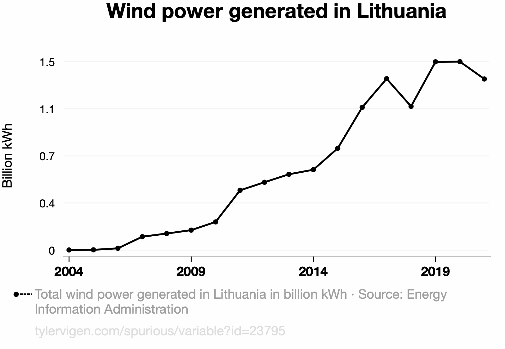
wind speed / power generated by wind turbine
soil C:N ratio / bacterial biomass / soil water content / leaf litter decomposition rate

Function notation

✏️

Function notation

Single variable (univariate) function:

$f(x) = [expression\space containing \space x]$

Multivariate function:

$g(a,T,z)=[expression\space containing \space a, T, \space and \space z]$

Evaluating functions

We evaluate functions by plugging in values of the input variables.

✏️ Example:

Evaluate $g(x,t)=2.4x+0.5t^2$ at $x = 3$ and $t = 10$

Evaluating functions

We evaluate functions by plugging in values of the input variables.

✏️ Example:

Evaluate $g(x,t)=2.4x+0.5t^2$ at $x = 3$ and $t = 10$

$g(3, 10) = 2.4(3) + 0.5(10^2)= 57.2$

Graphs

Why graphs?

Graphs are a way for us to more easily process trends or patterns that may be more challenging to understand in a table or list.

Which looks better and is easier to understand?

The $xy$ coordinate system

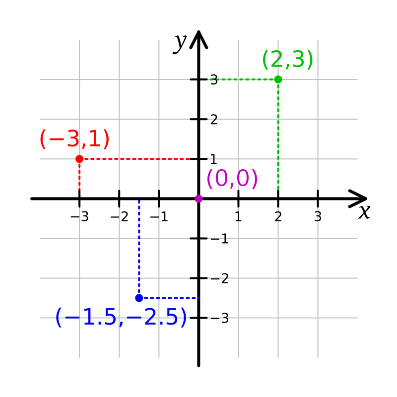
Graphs generally move in a 2-dimensional plane with a coordinate system using two axes:

$x$-axis (horizontal axis)
$y$-axis (vertical axis)

Axes units must be defined depending on the application.

We use pairs of numbers to place data:

A point on the $xy$ plane with coordinates $(a,b)$ means the point is located at $a$ on the $x$-axis and at $b$ on the $y$-axis.
Where would (2,-1) go on the graph?

We can join series of points to make graphs

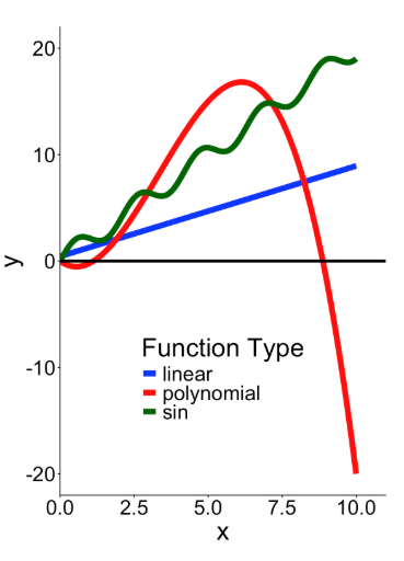
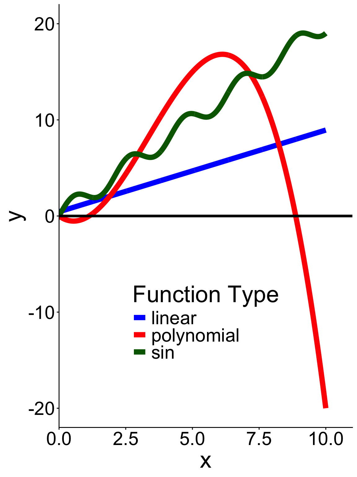
Functions on a single variable and a single output can be graphed

$\color{green}{y=sin(3x)+2x}$

$\color{red}{y=0.5x^3+x^2-5x}$

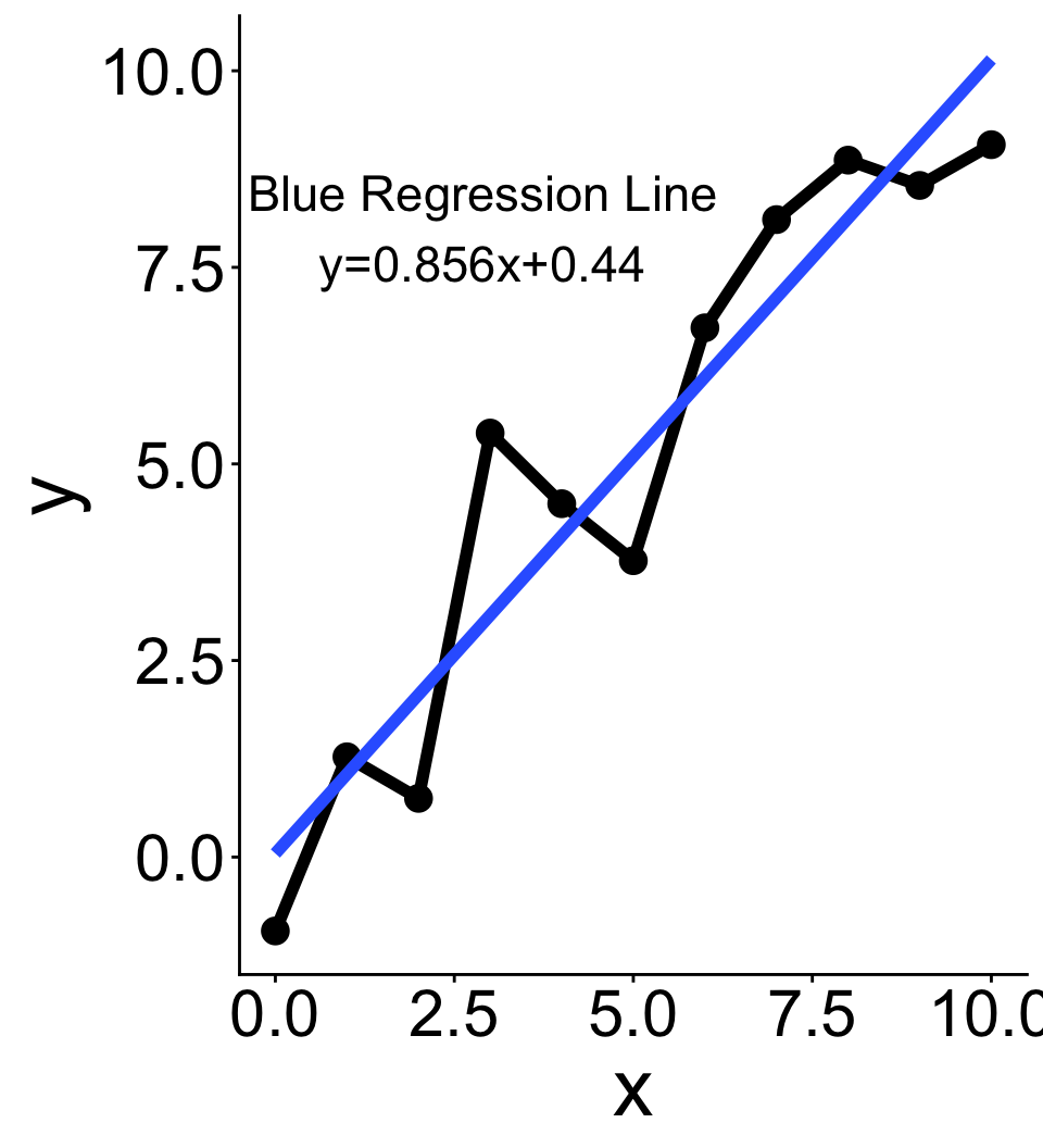
$\color{blue}{y=0.85x+0.44}$

Two key ingredients to graphs

Intercepts

$x$-intercept
- Where does the graph intersect the $x$-axis?
- In other words, for what values of $x$ do we have $(x,0)$ be part of the graph?

What are the intercepts of the polynomial function in red?

Two key ingredients to graphs

Intercepts

$x$-intercept
- Where does the graph intersect the $x$-axis?
- In other words, for what values of $x$ do we have $(x,0)$ be part of the graph?
$y$-intercept
- Where does the graph intersect the $y$-axis?
- In other words, for what value of $y$ do we have $(0,y)$ be part of the graph?

What are the intercepts of the polynomial function in red?

Understanding graphs

When you look at graphs, the first things you should ask:

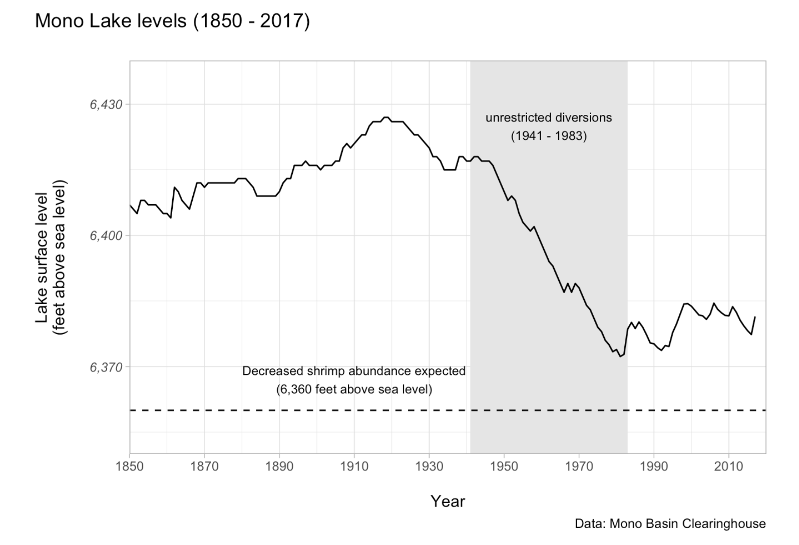
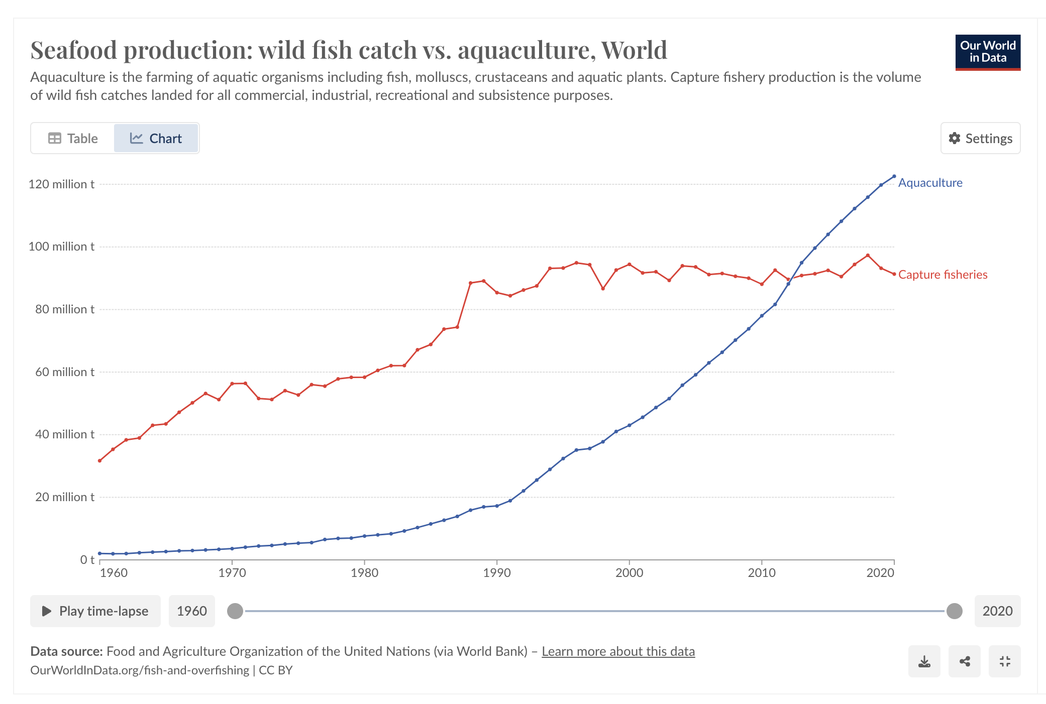
What variables are being plotted (e.g. x- & y-axis, including units)?

What values are plotted (e.g. raw values, transformed, means, etc.)?

What are the overall takeaways and am I understanding them responsibly?

Reading graphs (in general)

“On the x-axis we have [x-variable] measured in [units] and on the y-axis the the [y-variable] measured in [units]. This figure shows the [change/pattern/relationship] between [x-variable] and [y-variable]. Overall [overall statement of pattern / trend / findings].”

Reading graphs (in general)

“On the x-axis we have [x-variable] measured in [units] and on the y-axis the the [y-variable] measured in [units]. This figure shows the [change/pattern/relationship] between [x-variable] and [y-variable]. Overall [overall statement of pattern / trend / findings].”

Source: TylerVigen.com

Reading graphs practice

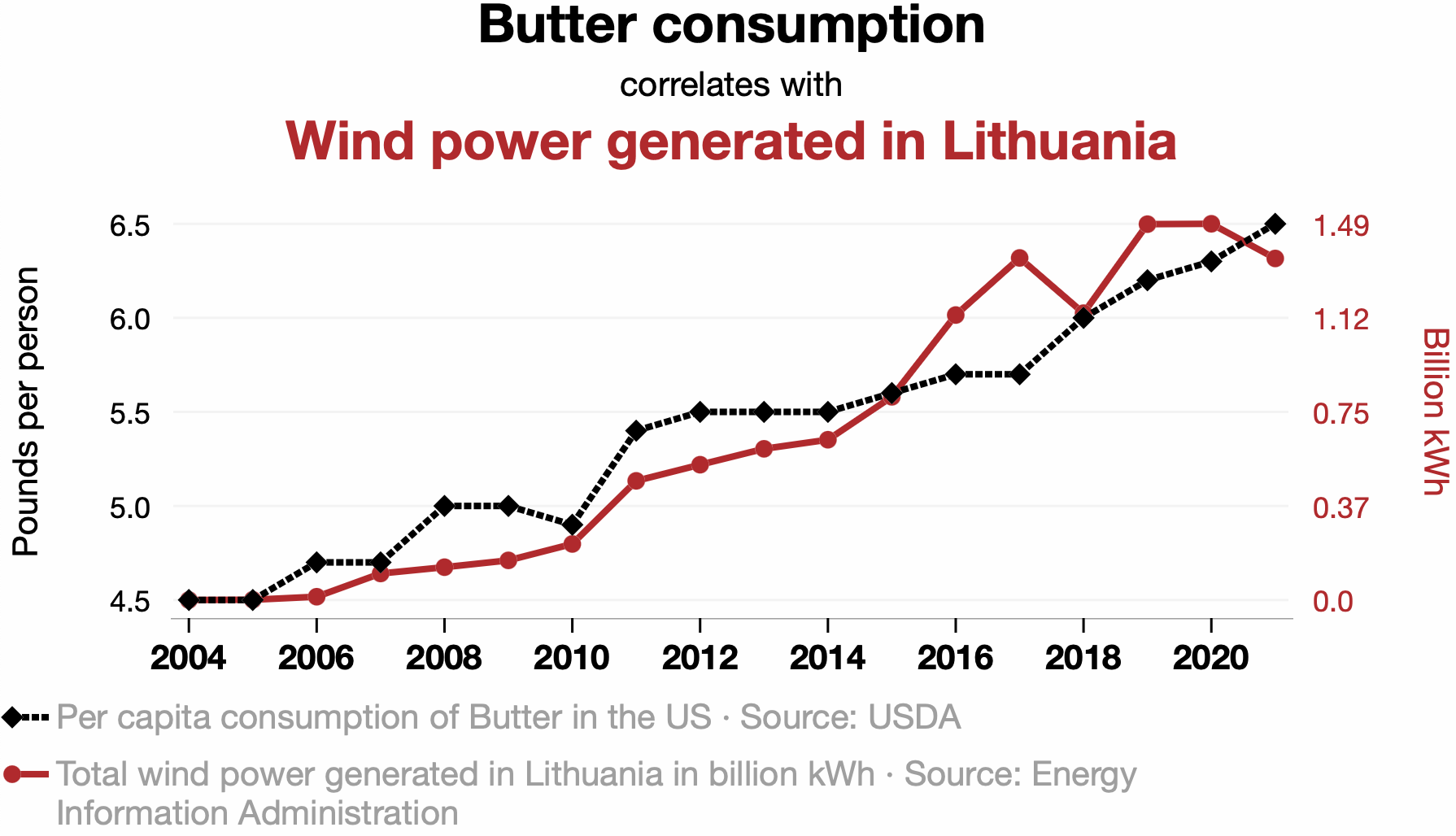
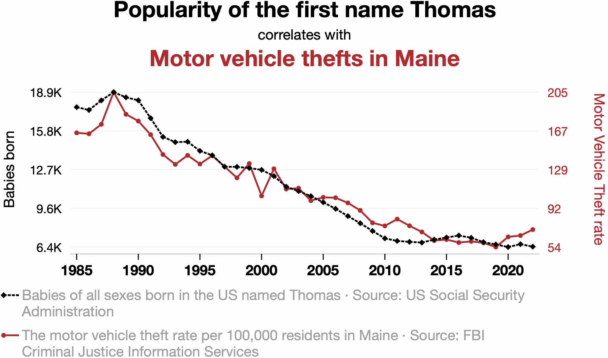
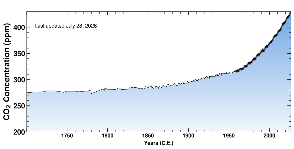
💬 Partner 1 gets to read the graph for the first variable.

“On the x-axis we have [x-variable] measured in [units] and on the y-axis the the [y-variable] measured in [units]. This figure shows the [change/pattern/relationship] between [x-variable] and [y-variable]. Overall [overall statement of pattern / trend / findings].”

Reading graphs practice

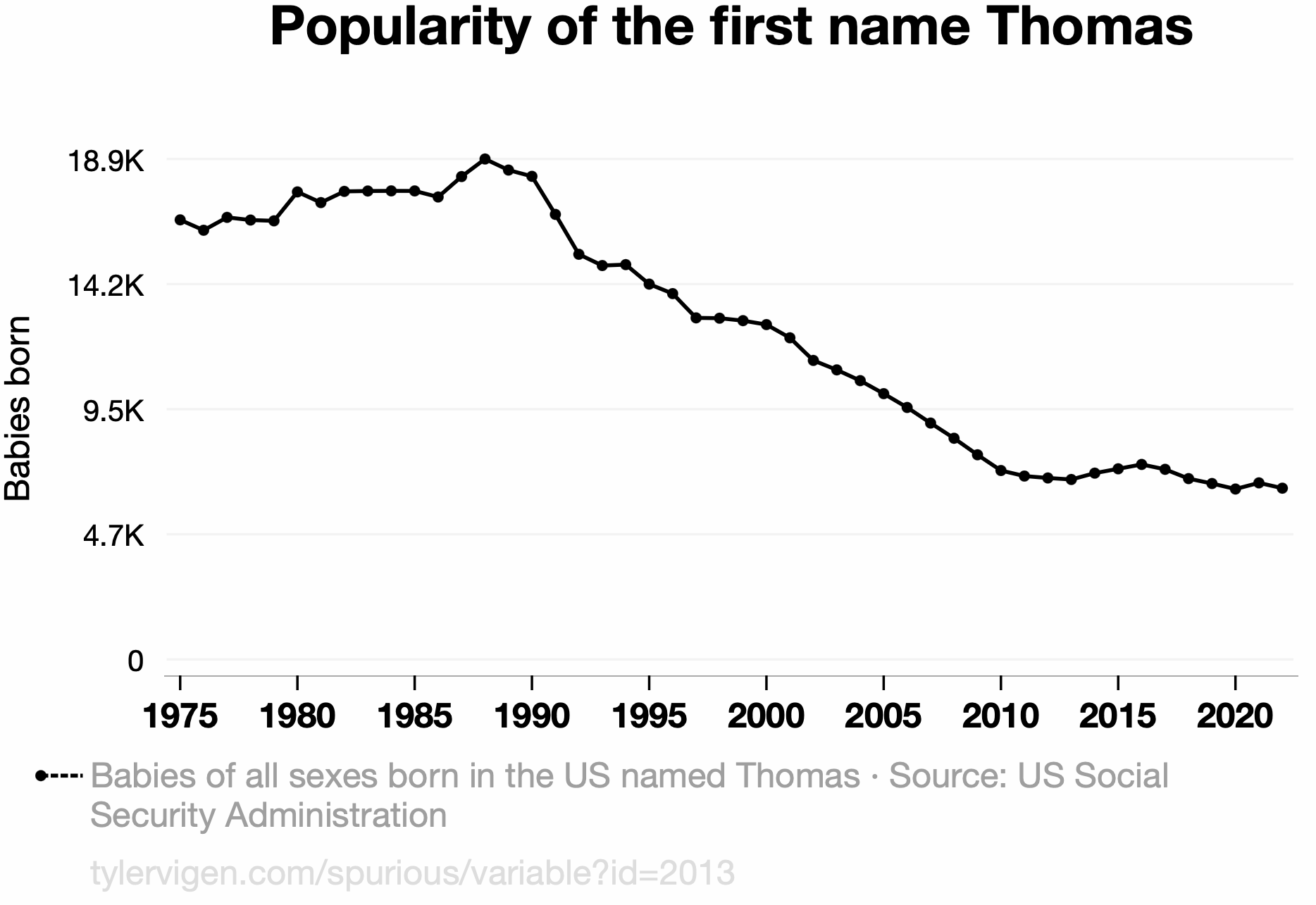
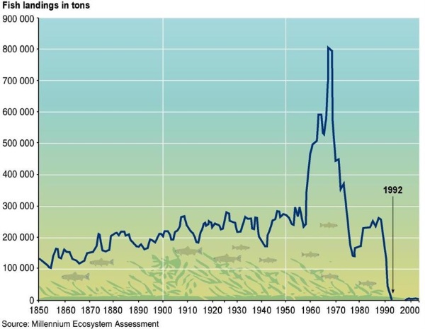
💬 Partner 2 gets to read the plot for the second variable, provide context for the data, and hypothesise an explanation.

“On the x-axis we have [x-variable] measured in [units] and on the y-axis the the [y-variable] measured in [units]. This figure shows the [change/pattern/relationship] between [x-variable] and [y-variable]. Overall [overall statement of pattern / trend / findings].”

Reading graphs practice

Let’s take a 5 minute break

image: Flaticon.com

The exponential function

The number $e$

The number $e$ is a constant in mathematics, it is approximately $e\approx 2.72$, but really its decimals continue infinitely without any pattern:

$e = 2.71828182845904523536...$

It’s exact value can be described as \[ e = 1 + 1 + \frac{1}{1*2} + \frac{1}{1*2*3} + \frac{1}{1*2*3*4} + \frac{1}{1*2*3*4*5} + ... \]

Like any other number, $e$ follows normal power properties:

\[ \begin{align} e^x\cdot e^y &=& ?\\ \frac{1}{e^x} &=& ?\\ \frac{e^x}{e^y} &=& ?\\ (e^x)^r &=& ? \end{align} \]

✏️ Take a moment to write these with a single exponent.

The number $e$

The number $e$ is a constant in mathematics, it is approximately $e\approx 2.72$, but really its decimals continue infinitely without any pattern:

$e = 2.71828182845904523536...$

It’s exact value can be described as \[ e = 1 + 1 + \frac{1}{1*2} + \frac{1}{1*2*3} + \frac{1}{1*2*3*4} + \frac{1}{1*2*3*4*5} + ... \]

Like any other number, $e$ follows normal power properties:

\[ \begin{align} e^{x+y}&=&e^x\cdot e^y \\ e^{-x}&=&\frac{1}{e^x}\\ e^{x-y}&=&\frac{e^x}{e^y}\\ e^{rx}&=&(e^x)^r \end{align} \]

The exponential funciton

The exponential function $e^x$ is the number $e$ raised to the $x$ power.

In function notation you may sometimes see it as

\[ f(x) = e^x \ \ \text{ or } \ \ \text{exp}(x).\]

Why is the exponential function so common?

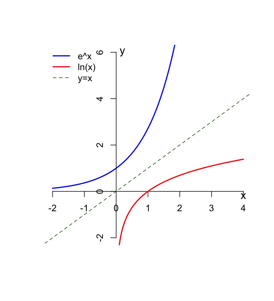
One reason: Exponential trends show up a LOT in environmental science (the proportional change is the same over each time span)
Math reason: Turns out it’s a very useful value for calculus

A real-world example:

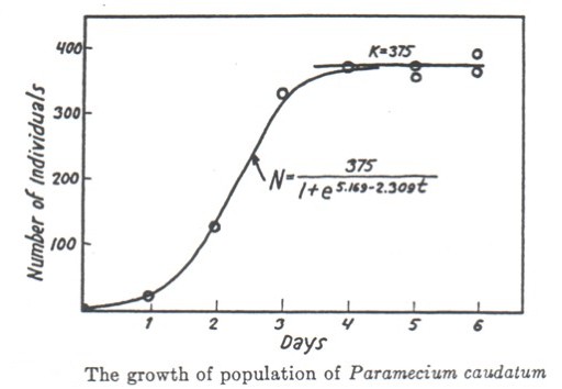
But populations can’t grow exponentially forever

Gause, G. F. 1934. The Struggle for Existence. Baltimore: Williams and Wilkins.

Logistic growth

\[N_t=\frac{K}{1+[\frac{K-N_0}{N_0}]e^{-rt}}\]

Where $N_t$ is the population size at time $t$, $K$ is the carrying capacity, $N_0$ is the initial population size, and $r$ is a growth rate.

✏️ What should be the value of the formula when $t=0$? Confirm your answer by substituting.

We should always understand the components of formulas and equations - both conceptually and mathematically.

Logistic growth: Example

What is \[N_t=\frac{K}{1+[\frac{K-N_0}{N_0}]e^{-rt}}\] when t = 0?

Solution

\[ \begin{aligned} N_0 &= \frac{K}{1+[\frac{K-N_0}{N_0}]e^{-r(0)}} &\text{Substitute } t=0 \\ &= \frac{K}{1+[\frac{K-N_0}{N_0}](1)} &e^{0}=1 \\ &= \frac{K}{\frac{N_0 + (K-N_0)}{N_0}} &\text{Combine terms in the denominator} \\ &= \frac{K}{\frac{K}{N_0}} &N_0 + (K-N_0) = K \\ &= N_0 \end{aligned} \]

Logistic growth

\[N_t=\frac{K}{1+[\frac{K-N_0}{N_0}]e^{-rt}}\]

Why might we expect logistic growth for many populations?
What variables besides time would influence the actual population?

Logarithms

$\log_a(b)$ is the exponent you need to raise $a$ to get a value of $b$

For example:

$\log_2(8)=x$ asks “to what power do I have to raise 2, to get a value of 8?”
$\log_{105}(1)=x$ asks “to what power do I have to raise 105, to get a value of 1?”

Natural logarithms

✏️

Natural logarithms

If $y>0$, then $\ln(x)$ is the exponent you need to raise $e$ to in order to get $y$.

This means:

\[ \begin{align} \ln(e^x) &= x \\ e^{\ln(y)} &= y \end{align} \]

In other words, $\ln(x)$ is the inverse of the exponential function $e^x$.

✏️ Examples

$\ln(e^3)$
$\ln(\frac{1}{e})$
$\ln(1)$
$\ln(0)$
$\ln(-7)$

Natural logarithms

If $y>0$, then $\ln(x)$ is the exponent you need to raise $e$ to in order to get $y$.

This means:

\[ \begin{align} \ln(e^x) &= x \\ e^{\ln(y)} &= y \end{align} \]

In other words, $\ln(x)$ is the inverse of the exponential function $e^x$.

Examples

$\ln(e^3) = 3$ because 3 is the power of $e$ needed to get $e^3$.
$\ln(\frac{1}{e}) = \ln(e^{-1}) = -1$
$\ln(1) = 0$ because 0 is the exponent we need to raise $e$ to to get 1
$\ln(0)$ does not exist, because there’s no number we can raise $e$ to to get 0
$\ln(-7)$ does not exist, because $e$ to any number always be positive

Natural log properties

✏️

Natural log properties

Properties

$\ln (e^x)=x$

$\ln(xy)=\ln x+\ln y$

$\ln(\frac{x}{y})=\ln x-\ln y$

$\ln(x^y)=y \ln x$

Using logarithms to solve equations

✏️ Solve for $t$ in the equation $Pe^{rt} = A$.

Properties

$\ln (e^x)=x$

$\ln(xy)=\ln x+\ln y$

$\ln(\frac{x}{y})=\ln x-\ln y$

$\ln(x^y)=y \ln x$

Using logarithms to solve equations

✏️ Solve for $t$ in the equation $Pe^{rt} = A$.

\[ \begin{align} Pe^{rt} &= A \\ e^{rt} & = \frac{A}{P} \\ rt &= \ln\left(\frac{A}{P}\right) \\ t &= \frac{\ln(A)-\ln(P)}{r} \end{align} \]

Linear functions

Linear functions: slope-intercept form

✏️

Linear functions: slope-intercept form

Easiest model to describe linear relationship between two variables!

\[ \huge \begin{align} \underbrace{y}_{\text{output}}=\overbrace{m}^{\text{Slope}}\underbrace{x}_{\text{input}}+\overbrace{b}^{\text{$y$ intercept}} \end{align} \]

Finding the equation of a line

✏️

Finding the equation of a line

Given two points $(x_1, y_1)$ and $(x_2, y_2)$ on the line:

Find $m$, the slope, by using the two points:

\[ m=\frac{\Delta y}{\Delta x}=\frac{y_2-y_1}{x_2-x_1}. \]

Find $b$, the y-intercept:

Since $(x_1, y_1)$ is on the line, it satisfies:

\[y_1 = mx_1+ b.\] We can solve for $b$ to obtain:

\[b = y_1 - mx_1.\]

Equation of a line: practice

Find the equation of the line that:
1. passes through $(3,5)$ and $(2,-1)$.
2. passes through $(2,-5)$ and has $x$-intercept equal to 4.
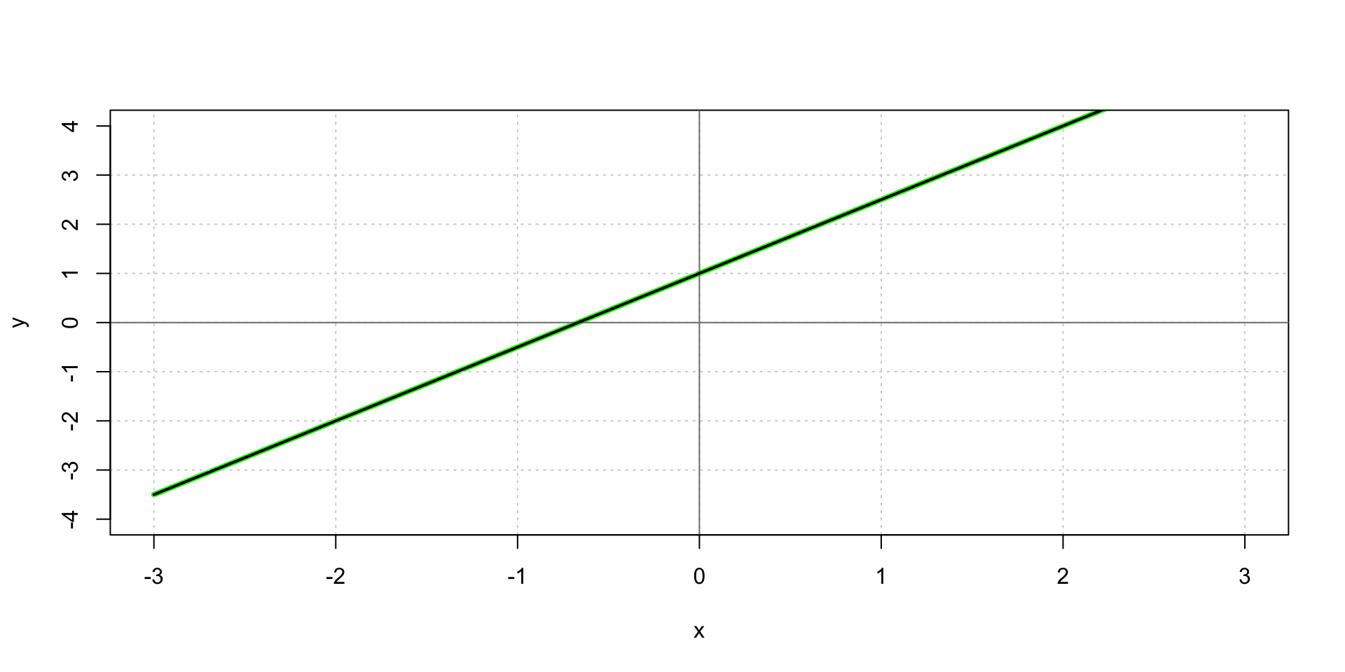
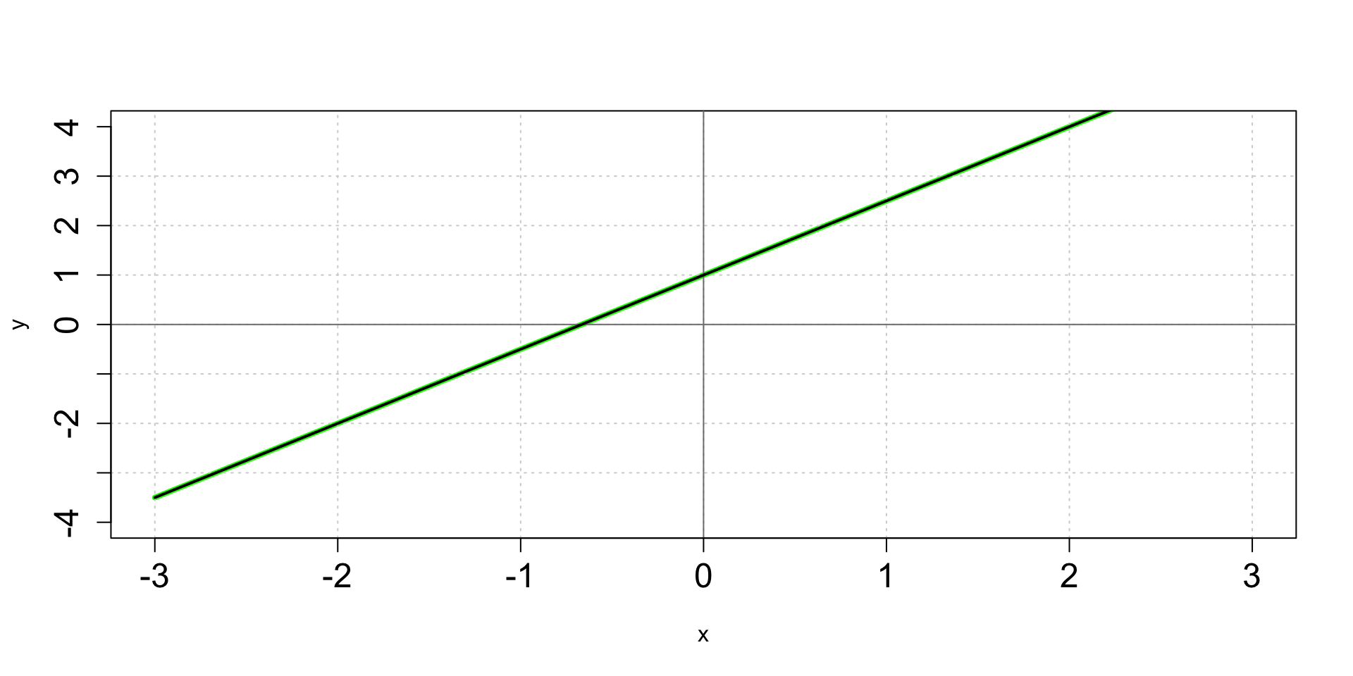
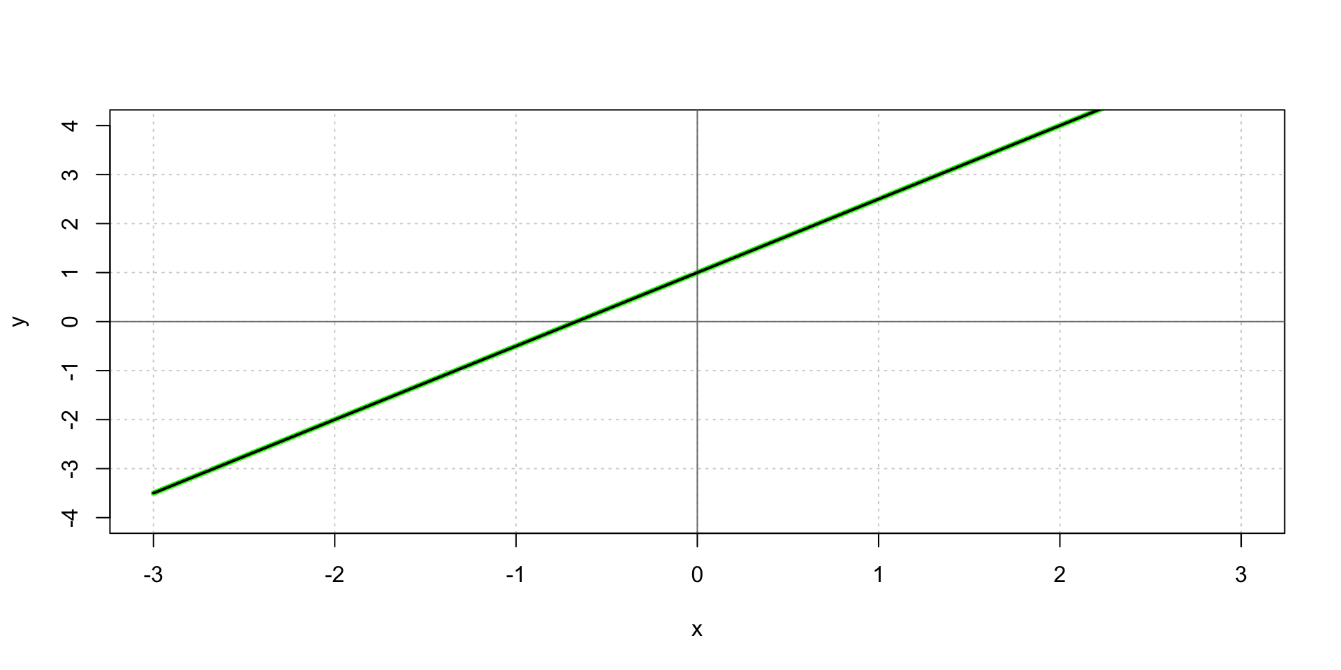
3. has the following graph:

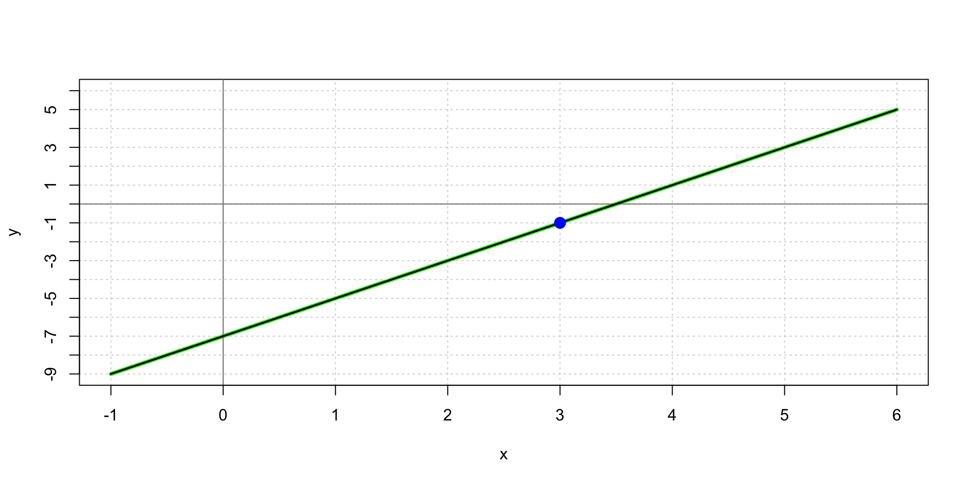
- Make a graph showing the line that passes through (3,-1) and has slope equal to 2.

Equation of a line: practice

A. Find the equation of the line that passes through $(3,5)$ and $(2,-1)$.

✏️ Let’s see a solution.

Equation of a line: practice

B. Find the equation of the line that passes through $(2,-5)$ and has $x$-intercept equal to 4.

✏️ Let’s see a solution.

Equation of a line: practice

C. Find the equation of the line that has the following graph:

✏️ Let’s see a solution.

Solutions

Passes through $(3,5)$ and $(2,-1)$:

\[ \begin{aligned} m &= \frac{5-(-1)}{3-2} = 6 &\text{Compute the slope} \\ y - 5 &= 6(x-3) &\text{Point-slope form using (3,5)} \\ y &= 6x - 13 &\text{Simplify} \end{aligned} \]

Passes through $(2,-5)$ and has $x$-intercept equal to 4:

\[ \begin{aligned} m &= \frac{0-(-5)}{4-2} = \frac{5}{2} &\text{Compute the slope using the } x\text{-intercept } (4,0) \\ y - 0 &= \frac{5}{2}(x-4) &\text{Point-slope form} \\ y &= \frac{5}{2}x - 10 &\text{Simplify} \end{aligned} \]

Has the given graph: $y = \frac{3}{2}x+1$

\[ \begin{aligned} \text{slope} &= \frac{\text{rise}}{\text{run}} = \frac{3}{2} &\text{Read from the graph} \\ y\text{-intercept} &= 1 &\text{Read from the graph} \\ y &= \frac{3}{2}x + 1 &\text{Equation of the line} \end{aligned} \]

Solutions

Make a graph showing the line that passes through (3,-1) and has slope equal to 2.

✏️ Let’s see a solution.

\[ \begin{aligned} y - (-1) &= 2(x-3) &\text{Point-slope form} \\ y &= 2x - 7 &\text{Simplify} \end{aligned} \]

Interpreting the slope

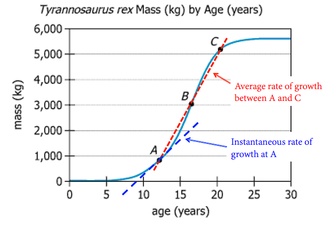
Slope (average)

Sometimes, it can be useful to find the average rate of change of a function.

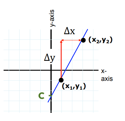
Between any two points $(x_1,y_1)$ and $(x_2,y_2)$ on the graph of a function, the slope is found by:

\[m=\frac{\Delta y}{\Delta x}=\frac{y_2-y_1}{x_2-x_1}\]

Same idea as in a line!

Slope represents rate of change

Ice-core data before 1958. Mauna Loa data after 1958.

Source:The Keeling Curve

Get into the practice of saying the meaning out loud

As if you’re explaining it to someone unfamiliar with the data
Including units
Without overstating certainty

For example:

“Between 1972 and 2020 the price of hobbit homes increased by an average of $2,450 per year”

differs from

“Between 1972 and 2020 the price of hobbit homes increased by $2,450 per year.”

The average slope of a continuous function rarely tells the whole story

Slope can be average or instantaneous

Rise over run can always be used to find average rate of change between two parts of a graph

Instantaneous rate of change leads us to ✨calculus✨.

End of day 1!

What we covered today

🔢 Algebra review
🗺️ Solving equations
✖️ Exponents
📐 Polynomials
🌡 Units
🧩 Definition of functions
📊 Graphing
💬 Reading graphs
🌱 The number e and exp()
🐰 Logistic growth
🪵 Natural logarithms
📈 Linear functions
↗️ Slope as a rate of change