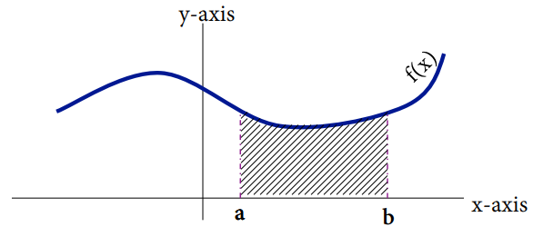
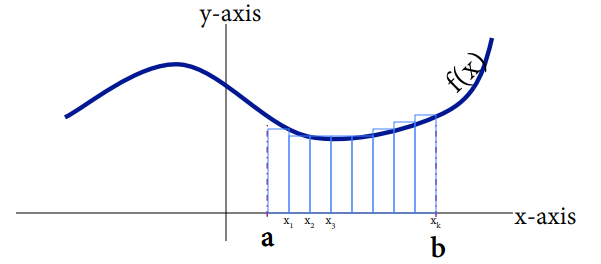
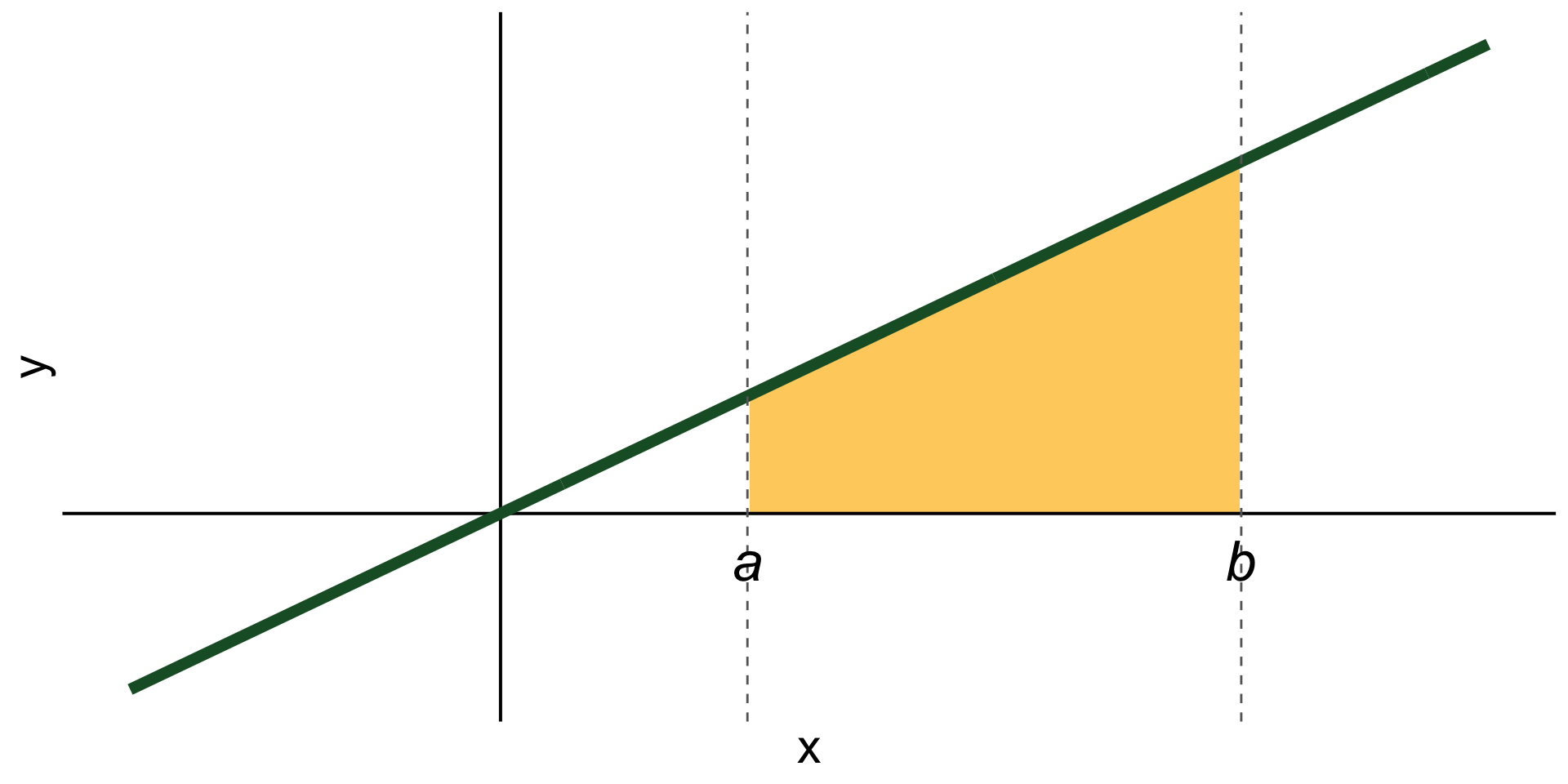
Areas of rectangles are easy to find (base times height!). We can approximate the area by adding the area of rectangles under the curve.
Example
Approximate the area under the curve from \([-3,3]\) with \(\Delta x=2\) and \(k=3\).
✏️
x
y
-3
71
-1
73
1
51
3
53
Riemann sums
Divide the interval \([a,b]\) into \(k\) subintervals of width \(\Delta x\).
The endpoints of those intervals will give you a series of \(x\) values: \(x_0, x_1, \ldots, x_k\).
Multiply \(f(x_1)\Delta x\) to get the the area of the first rectangle.
Repeat the same steps above, now starting with \(x_2\) as the bottom right corner of the next rectangle. Repeat until you cover the area with rectangles of width \(\Delta x\).
Sum up the area of all \(k\) rectangles.
\[
R(f(x), \Delta x)= \underbrace{f(x_1)\Delta x+f(x_2)\Delta x+...f(x_k)\Delta x}_{\text{Sum of area of rectangles with width $\Delta(x)$} }
\]
This is called a Riemann Sum.
Finer and finer Riemann sums
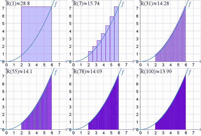
What if we try to make \(\Delta x\) (the width of the rectangles) really small? So we let \(\Delta x \to 0\). This will make the number of rectangles under the curve go to infinity.
Our estimation of the area will get better and better with more rectangles.
Finer and finer Riemann sums
What if we try to make \(\Delta x\) (the width of the rectangles) really small? So we let \(\Delta x \to 0\). This will make the number of rectangles under the curve go to infinity.
Our estimation of the area will get better and better with more rectangles.
Take the area calculation we did before, but let \(\Delta x \to 0\)\[
\large
\begin{align}
\text{True Area} &= \lim_{\Delta x \to 0}R(f(x),\Delta x) \\
&= \int^b_af(x)dx
\end{align}
\]
We formally call this the integral of \(f(x)\) from \(a\) to \(b\) with respect to \(x\).
How do we calculate integrals?
Taking infinite sums is impossible by hand
Luckily, integrals and derivatives are related in a very useful way:
How do we calculate integrals?
Taking infinite sums is impossible by hand
Luckily, integrals and derivatives are related in a very useful way:
If we integrate a derivative, we should get the same function back as the original vice-versa:
\[
\begin{align}
\frac{d}{dx}\left[\int f(x)dx\right]&=f(x) &\text{Differentiation is the inverse of integration}
\end{align}
\]
\[
\begin{align}
\int f'(x)&=f(x)+C &\text{Integration is the inverse of differentiation}
\end{align}
\]
To find the integral of \(\int f(t) dt\) we need to find a function \(F(x)\) whose derivative is \(f(x)\).
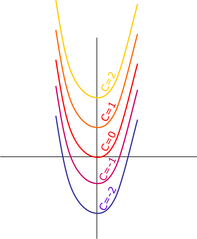
Where did that \(C\) come from?
Example
✏️
Where did that \(C\) come from?
Example
Find \(\int 2x-4\).
To find \(\int 2x-4\) we need to find a function whose derivative is \(2x-4\). What could it be?
If we integrate, we’ll have \(\int 2x-4 = x^2-4x+C\).
There is no way of knowing what the \(C\) should be without additional information
\(C\) is the \(x\)-intercept and we would have we have to solve for it with an initial value problem.
When you take an integral, the function in it can be in terms of any variable. This is just notation and it does not affect the result of the integration:
\[\int f(x) dx = \int f(t) dt = \int f(u) du.\]
Integration rules (1)
Sum and Difference Rules
✏️
Integration rules (1)
Sum and Difference Rules
The integral of a sum is equal to the sum of the integrals:
\[
\int[f(x)+g(x)]dx=\int f(x)dx+\int g(x)dx
\]
The integral of the difference is equal to the difference of the integrals:
\[\int[f(x)-g(x)]dx=\int f(x)dx-\int g(x)dx \]
Integration rules (2)
Constant Rule
✏️
Integration rules (2)
Constant Rule
When a function is mulitplied by a constant, the constant can be taken out to multiply the integral:
\[
\int cf(x)dx=c\int f(x)dx
\]
Integration rules (3)
Power Rule
✏️
Integration rules (3)
\(\int x^n dx\) is a function whose derivative is \(x^n\).
To find the \(C\) term in the integral, we need extra information
Often times that comes from being given an initial value
This means being given some value of the function, e.g. \(y(0)=a\) or \(y(12)=b\)
We use this information to solve for what \(C\) should be
Example
✏️ The marginal cost of producing \(x\) units of a product is:
\[
\frac{dC}{dx}=25-0.02x
\]
Where \(C\) is the cost (in dollars), and \(x\) is the number of units produced. Given that producing 2 units of product costs $10, what is the complete cost equation?
Example
✏️ The marginal cost of producing \(x\) units of a product is:
\[
\frac{dC}{dx}=25-0.02x
\]
Where \(C\) is the cost (in dollars), and \(x\) is the number of units produced. Given that producing 2 units of product costs $10, what is the complete cost equation?
We can integrate to find the original cost function \(C\):
\[C(x) = \int \frac{dC}{dx} dx = \int 25-0.02x.\]
Then: \[
\begin{align}
\int 25-0.02x =&25x-\frac{.02x^2}{2}+D & \text{Solve with Power Rule}\\
10&=25(2)-\frac{0.02(2)^2}{2}+D &\text{ Sub in $x=2$}\\
-39.96&=D\\
C(x)&=25x-\frac{0.2x^2}{2}-39.96
\end{align}
\]
Let’s take a 5 minute break
image: Flaticon.com
Definite integrals
Indefinite vs. definite integrals
✏️
Indefinite vs. definite integrals
We have been working with indefinite integrals.
\[
\int f(x)dx
\]
This means there are no integration bounds and we need initial values to find integration constants.
Definite integrals have start and end values \(a\) and \(b\):
\[\int_a^b f(x) dx.\]
To find the area under the curve along an interval \([a,b]\), evaluate the antiderivative at the endpoints and subtract them.
A model for the rate of change in ozone concentrations over time between 1962-1984 is given by \(\frac{dC}{dt}=2t+20\), where \(C\) is the ozone concentration (ppm) and \(t\) is the elapsed time in years since 1962. Given that in 1964 the ozone concentration was 30 ppm, what was the ozone concentration in 1982?
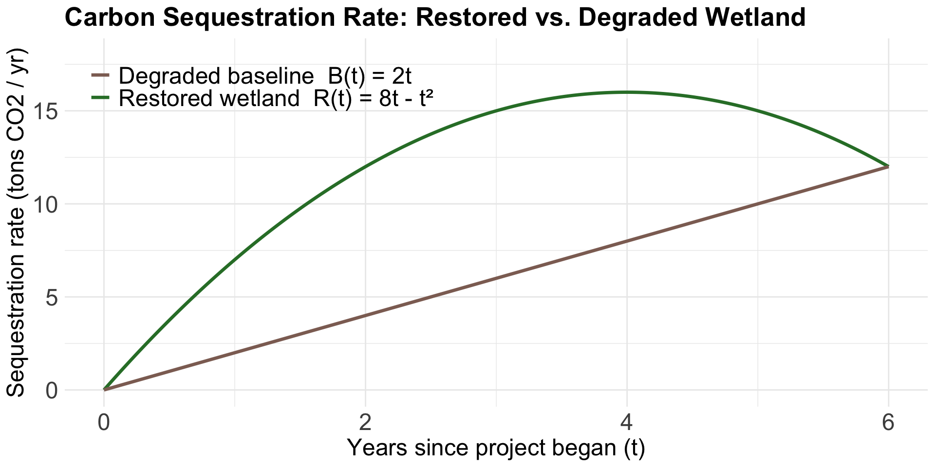
A coastal wetland restoration project is being evaluated against a “do-nothing” baseline where the wetland is left degraded. Ecologists model the carbon sequestration rate (tons CO₂ / year) as a function of years since the project began, \(t\):
Restored wetland: \(R(t) = 8t - t^2\)
Degraded baseline: \(B(t) = 2t\)
Both models are valid for \(0 \le t \le 6\). What is the total additional carbon sequestered by the restored wetland over the 6-year period?
Write your answers as full sentences with units!
Solution (2)
A model for the rate of change in ozone concentrations over time between 1962-1984 is given by \(\frac{dC}{dt}=2t+20\), where \(C\) is the ozone concentration (ppm) and \(t\) is the elapsed time in years since 1962. Given that in 1964 the ozone concentration was 30 ppm, what was the ozone concentration in 1982?
✏️
Solution (2)
Given: \[\frac{dC}{dt} = 2t + 20\]
Integrate: \[\int dC = \int (2t + 20)\,dt\]
\[C(t) = t^{2} + 20t + D\]
Initial condition: \[C(2)=30 \ \ \text{(since 1964 is 2 years after 1962)}\]
\[30 = 2^{2} + 20\cdot 2 + D\]
\[D = 30 - 44 = -14\]
Thus: \[C(t) = t^{2} + 20t - 14\]
Evaluate at \(t=20\) (1982):
\[C(20) = 20^{2} + 20\cdot 20 - 14\]
\[= 400 + 400 - 14\]
\[= 786 \text{ ppm}\]
Solution (3)
A coastal wetland restoration project is being evaluated against a “do-nothing” baseline where the wetland is left degraded. Ecologists model the carbon sequestration rate (tons CO₂ / year) as a function of years since the project began, \(t\):
Restored wetland: \(R(t) = 8t - t^2\)
Degraded baseline: \(B(t) = 2t\)
Both models are valid for \(0 \le t \le 6\). What is the total additional carbon sequestered by the restored wetland over the 6-year period?
✏️
Solution (3)
✏️
Solution (3)
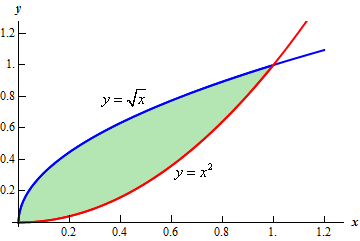
The toal carbon sequestered in each scenario is given by the area under the curve of the corresponding sequestration rate.
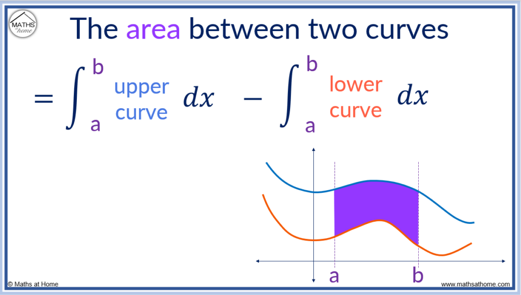
So the total additional carbon sequesterd is represented by the area between the two sequestration rate curves.
Differential equations help us understand changing environments
For some natural phenomena it can be easier to describe them in terms of derivatives than give an explicit function.
By specifying how something changes, we are describing a process or behavior over time.
Examples:
Describing population dynamics
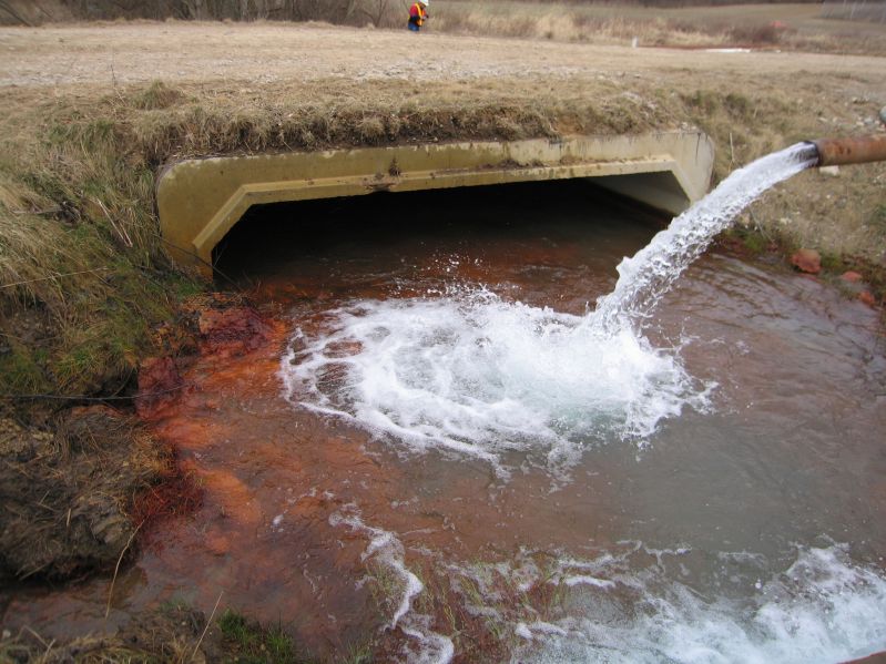
Groundwater transport of absorbed contaminants
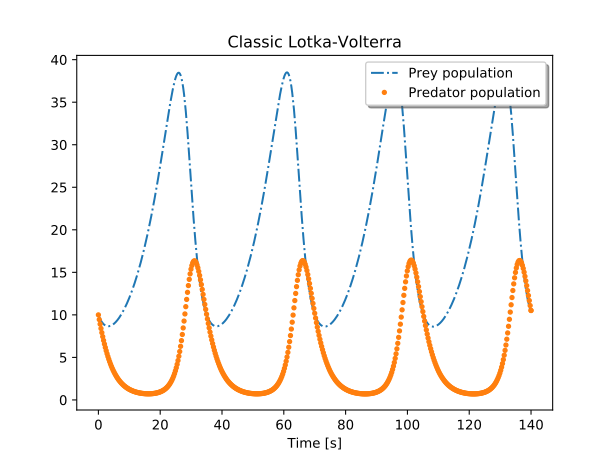
Example: Lotka-Volterra (predator-prey) equations
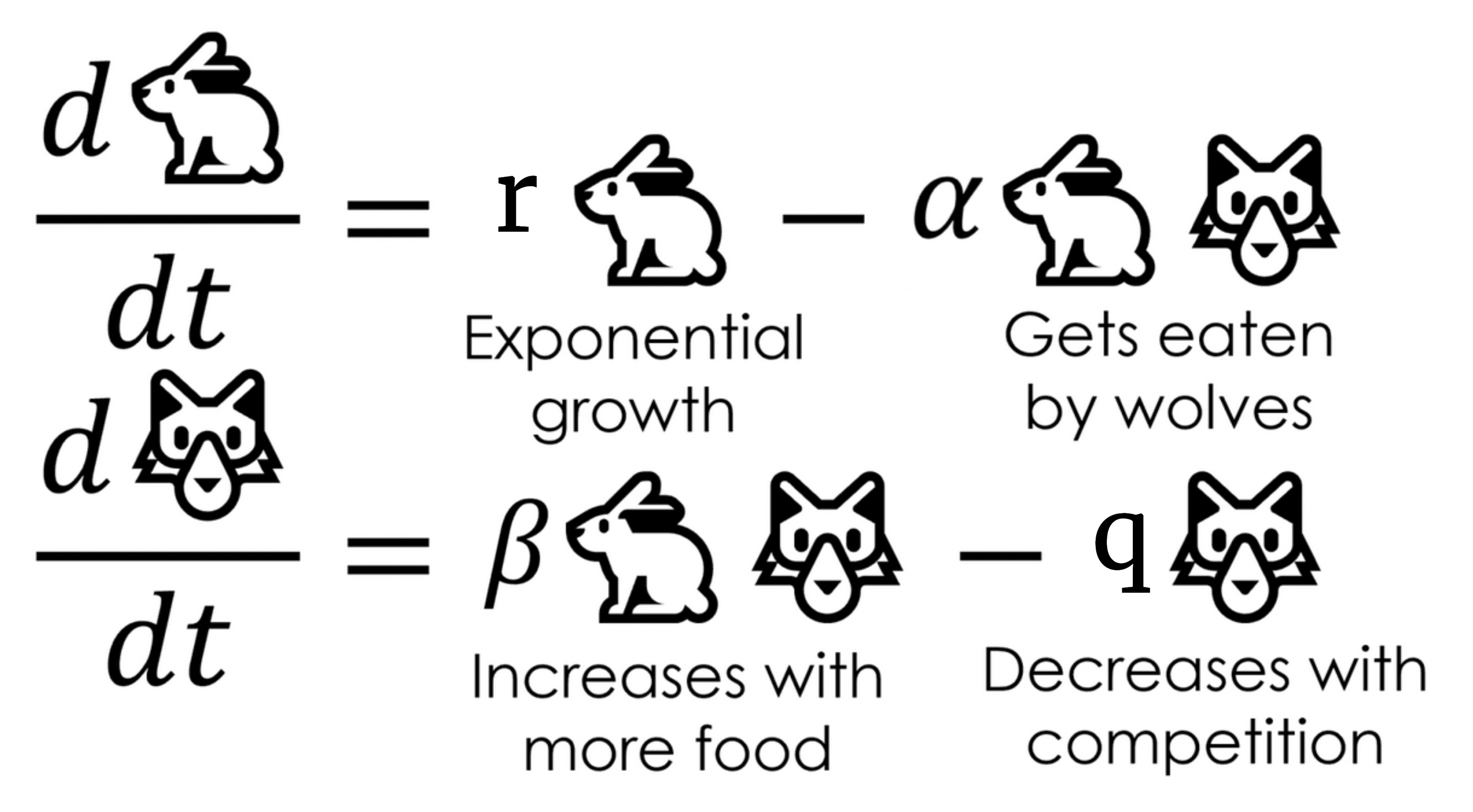
Prey: \(\frac{dV}{dt}=r V-\alpha VP\)
Predator: \(\frac{dP}{dt}=\beta VP - qP\)
Where:
\(V\) is number of prey (e.g. rabbits)
\(P\) is number of predators (e.g. wolves)
\(r, \alpha, \beta, q\) are positive parameters
What do the different pieces of the equation mean?
Interpretation of prey equation:
\[\frac{dV}{dt}=r V-\alpha VP\]
The pieces:
\(\frac{dV}{dt}\): Rate of growth / decline in prey abundance
\(r V\): Population growth (without loss due to predation (assumes predators are the only force limited the growth of the prey population), where \(r\) is the intrinsic rate of increase)
\(-\alpha VP\): Population loss due to predation (where \(\alpha\) is the capture efficiency of the predator)
Interpretation of predator equation:
\[\frac{dP}{dt}=\beta VP - q P\]
The pieces:
\(\frac{dP}{dt}\): Rate of growth / decline in predator population
\(\beta VP\): Predator population growth (where \(\beta\) is a measure of conversion efficiency, i.e. the ability of predators to convert each new prey into additional per capita growth rate for the predator population)
\(-q P\): Predator population loss (where \(q\) is the per capita death rate; positive population growth only happens when prey are present)
Or, in pictures:
Finding \(V(t)\) and \(P(t)\)?
Some differential equations can be solved analytically:
✏️
Some differential equations can be solved analytically:
\[\frac{dy}{dx}=y\]
Separate variables and integrate both sides:
\[\int\frac{1}{y}dy=\int1dx\]
Yielding:
\(ln(y)=x\) or \(y=e^x\)
Solving differential equations numerically
Find approximate solutions to differential equations when finding an analytical solution would be really challenging (…which is pretty often).
Instead, computers can numerically approximate solutions by predicting nearby values based on the slope.
There are many methods for solving differential equations numerically. You’ll do it programatically later on.