…because you should do it just one time.
A file path is a string of characters that points to a unique location in your computer where a file or folder either currently exists or will exist. Different sections of the path are separated by a path separator. A path separator can be a forward slash (/) in Mac OS or backward slash (\) in Windows/Linux.
In Mac OS, you can hold the Option and Shift keys and click on the item. In the pop-up window, you can then select “Copy [item name] as Pathname”.
In Windows and Linux, you can hold the Shift key and double click on the item. In the pop-up window, you can then select the “Copy as path”.
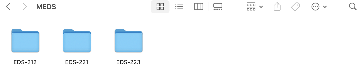
For ease of troubleshooting, set up your file organization like so:
…because you should do it just one time.
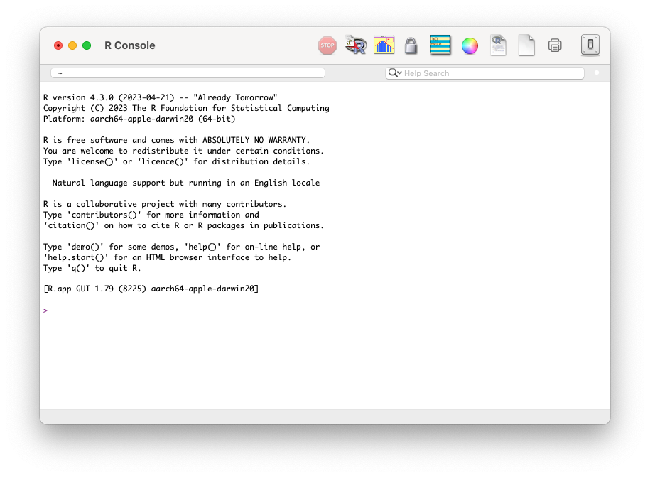
Always remember: R is the programming language. RStudio is the IDE.
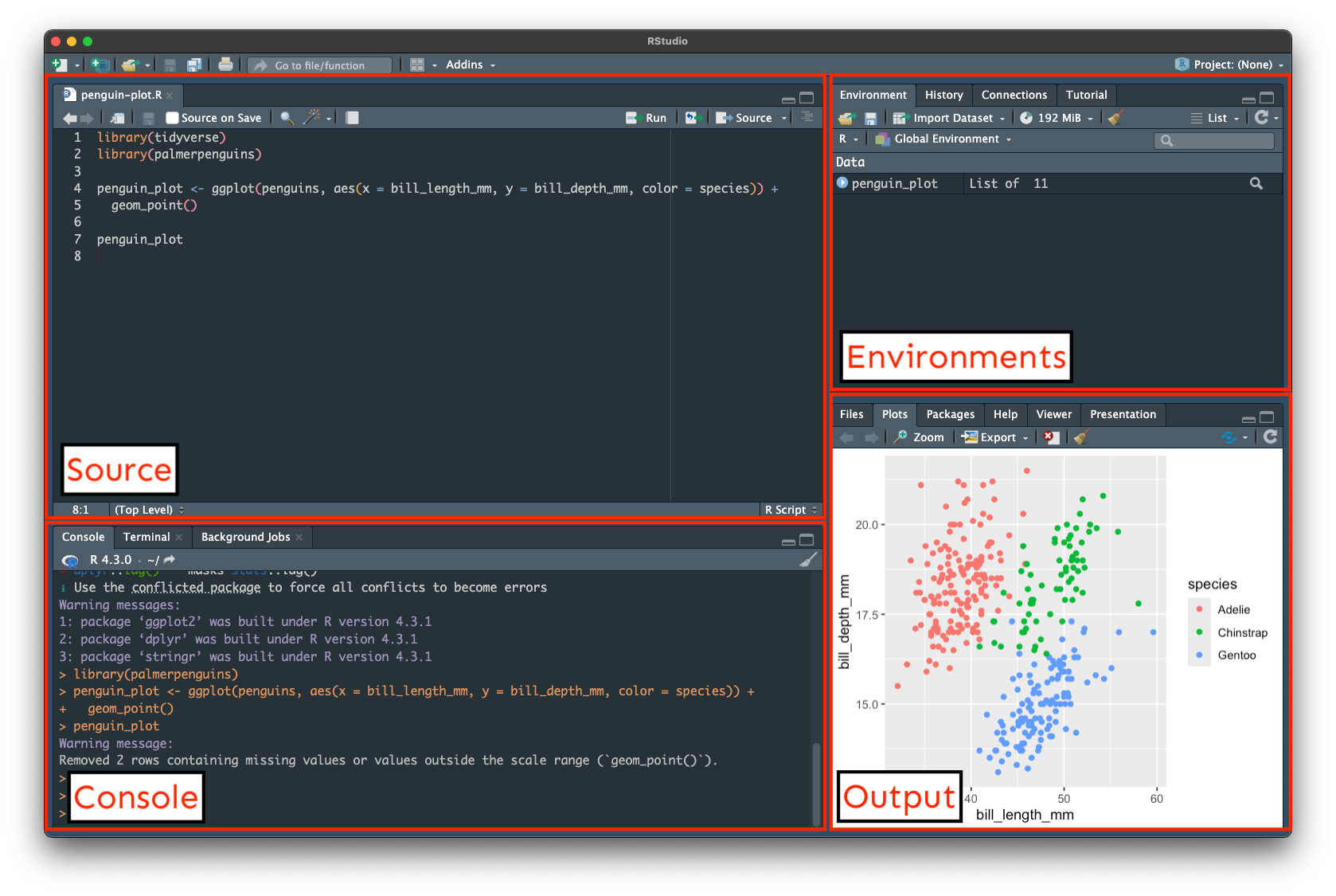
RStudio provides a nice user interface for data science, development, reporting, and collaboration (all of which you’ll learn about throughout the MEDS program) in one place. Note that while it’s called RStudio, it is a useful IDE for development in a number of languages and file types (check out some by clicking on File > New File, and seeing the multitude of options that RStudio suggests).
Let’s take a quick tour of the RStudio IDE, then customize it for fun and functionality:
You can check out the RStudio User Guide for additional information and helpful tips!
Next, let’s familiarize ourselves with some basic operations in the Console:
*, /, +, -, ^), as well as functions to perform calculations in the Console:RStudio Console
# perform calculations using operators:
7 * 11
21 / 3
1 + 1
4 - 3
4 ^ 2

# perform calculations using functions:
sqrt(4) # compute the square root?function_name. For example, try running, ?sqrt, in the Console
sqrt() computes the (principle) square root of x, \(\sqrt{x}\), and takes one argument, x. We must supply a value for the x argument in order for the function to execute. The Arguments section of the documentation tells us that x can be a numeric or complex vector or array. We can supply just our numeric value (e.g. 4), or explicitly include the argument name as well:RStudio Console
sqrt(4)
sqrt(x = 4)<-. Any objects (also called variables) will appear in the Environment tab. Use snake_case and always start object names off with a letter (and not a number). For example:RStudio Console
current_year <- 2024
class_num <- "EDS 212"
temp_c <- 17.4 If we want to save our code so that we can access / re-run it later (which, in most cases, you do!), we can instead write our code in an R script (rather than directly in the console):
Create a new R script by clicking on the new file button (top left corner of RStudio), then choosing R Script.
Create some variables to your script, then save it (to your EDS-212 folder). Run your code and see your variables appear in your Environment:
.R
# my variables ---
current_year <- 2024 # integer
class_num <- "EDS 212" # character string
temp_c <- 17.4 # numeric#
We’ll talk a lot about the importance of annotating your code (i.e. leaving notes so that collaborators, including future YOU, can better understand your code and decisions) throughout the MEDS program. Any text prefixed with a # is an “annotation” and will not be executed when you run your code.
Quarto is a publishing framework that lets you make all kinds of things (dashboards, websites, notebooks, slides, books, etc.) that combine markdown (plain text with added formatting), code, and outputs in one place - which makes it an incredible tool for reproducibility. Let’s make a Quarto document (New File (top left corner) > Quarto Document… > provide it with a title (e.g. My first Quarto doc!) and learn by doing.
Render your Quarto doc – when you first create a new Quarto doc, it’ll have some pre-populated content. Click the Render button at the top of your file (it’ll prompt you to save your file first – you can save this to your EDS-212 folder). This converts all the content first to plain markdown, then to the file output type that you select (the default, and the one we’ll use most often, is HTML)
Delete all the pre-populated content starting on line 6 (beneath the YAML gates, ---; more on YAML later)
Let’s add some of our own formatted content to the body of our Quarto doc, including:
#, ##, … to start the line)*, or dashes, -, to start lines)[text here!](link here))command/control + option + I. Try adding the same variables as before to your new code chunk, along with annotations (again, using the # symbol).command/control + enter/return, or using buttons buttons (Run button at the top right of your file, or the green play button on each individual code chunk)We’ll get into the weeds of functions in EDS 221. For now, we’ll create functions to quickly do repeated calculations, and to familiarize ourselves with function notation.
General function notation looks like this:
function_name <- function(argument_1, argument_2) {

  function_body

}
For example, let’s make a function to help us convert units of \(\frac{g}{cm^3}\) to \(\frac{kg}{ft^3}\), given that \(1 cm^3 = 3.531\times10^{-5}ft^3\)
\[\frac{g}{cm^3}*\frac{1 kg}{1000 g}*\frac{1cm^3}{3.531\times10^{-5}ft^3}\]
.qmd
convert_units <- function(value_g_cm3) {
  value_kg_ft3 = value_g_cm3 * (1 / 1000) * (1 / 3.531e-5)
  print(value_kg_ft3)
}.qmd
convert_units(50)[1] 1416.029If you are writing code reproducibly, you should be able to close the file you’re working in without stress. That’s because all of your stored objects - functions, variables, etc. - should be recreated by opening and re-running the code in your file. If you cannot do that, then your code is not reproducible.
That means that your scripted code is what is precious - and we want to build bomb-proof strategies for making sure it’s safe.
Which brings us to a critical lesson: Create things like you expect your computer to explode at any minute. Your computer is NOT a safe place. Where is? Someone away from your local computer…somewhere cloudlike and wonderful. Somewhere like GitHub (coming up soon!).
End interactive session 1A