End interactive session 2A
xxx_title2("text here")Derivatives by hand, in R, meet git & GitHub
Use the definition of the derivative:
\[\frac{df}{dx}=\lim_{h\to 0}\frac{f(x+h)-f(x)}{h}\]
\(f(x)=3x^2-x+1\)
\(=\lim_{h\to 0}\frac{3(x+h)^2-(x+h)+1-(3x^2-x+1)}{h}\)
\(=\lim_{h\to 0}\frac{3(x^2+2xh+h^2)-x-h+1-3x^2+x-1)}{h}\)
\(=\lim_{h\to 0}\frac{3x^2+6xh+3h^2-x-h+1-3x^2+x-1)}{h}\)
\(=\lim_{h\to 0}\frac{3h^2+6xh-h}{h}\)
\(=\lim_{h\to 0}3h+6x-1\)
\(=6x-1\)
\(G(t)=4-3t\)
\(=\lim_{h\to 0}\frac{4-3(t+h)-(4-3t)}{h}\)
\(=-3\)
\(f(x) = -3x^5+2x^3-12\)
\(\frac{df}{dx} = -(3)(5)x^4+(2)(3)x^2-0\)
\(\frac{df}{dx} = -15x^4+6x^2\)
\(\frac{dC}{dz} = 4.2 - (3)(8.7)z^2\)
\(\frac{dC}{dz} = -26.1z^2 + 4.2\)
\[B(t) = 0.4 + 0.035t^2\]
\(B(t) = 0.4 + 0.035t^2\)
\(B(4.5) = 0.4 + 0.035(4.5)^2\)
\(B(4.5) = 0.4 + 0.035(20.25)\)
\(B(4.5) = 0.4 + 0.70875\)
\(B(4.5) = 1.10875 \ grams\)
\(B(t) = 0.4 + 0.035t^2\)
\(\frac{dB}{dt} = 0 + (0.035)(2)t\)
\(\frac{dB}{dt} = 0 + (0.035)(2)(10)\)
\(\frac{dB}{dt} = 0.7 \ grams/hr\)
D()eds212-day2a# in a script)D() (and optionally, deriv()){ARTofR} to create beautifully-formatted section headers for your scripts
Just because we aren’t working in a Quarto document (where we can combine prose and code) doesn’t mean clear annotations and section headers aren’t important!
The {ARTofR} package is wonderful for creating clean titles, dividers, and block comments for your code. Install the RStudio Addin, or call {ARTofR} functions in your console to generate comments, copy to your clipboard, and paste into your scripts.
If you opt for the function / console approach:
library(ARTofR)) in your Console (rather than in your script/qmd file)xxx_ into your Console, which should pull up an auto fill list of options)xxx_title2("My section title")) into the console – the resulting divider is automatically copied to your clipboardFor example:
creates the header:
And:
creates the divider:
There are two functions, D() and deriv(), which can be used to compute the derivatives of expressions in R. Both accept two arguments, expr (an expression or formula) and name (the variable that the derivative will be carried out with respect to). We’ll focus primarily on using D(), but examples are provided for using deriv() as well:
D():D() computes the derivative of a simple expression. Let’s use D() to evaluate the same expression, \(5x^2\), again at \(x = 2.8\):
# Create an expression (right hand side of the equation) ----
my_expression <- expression(5 * x^2)

# Find the derivative of your expression with respect to x using `D()` ----
my_derivative <- D(expr = my_expression, name = "x")

# Check it out ----
my_derivative
5 * (2 * x)# Evaluate it at x = 2.8 ----
x <- 2.8
# Evaluate it! (value returned is slope) ----
eval(my_derivative)[1] 28deriv():deriv() (collapsed to save space):
Using deriv() is valuable when you encounter more complex scenarios where you need to evaluate both the function and it’s derivative(s). It can handle multivariate functions, and is useful in optimization contexts (so you may see this again in machine learning!). The code looks pretty similar to the example using D(), above, but it returns a bit more information in the output:
# Create an expression (right hand side of the equation) ----
my_expression <- expression(5 * x^2)

# Find the derivative of your expression with respect to x using `deriv()` ----
my_derivative <- deriv(expr = my_expression, name = "x")

# Check it out ----
my_derivative
expression({
.value <- 5 * x^2
.grad <- array(0, c(length(.value), 1L), list(NULL, c("x")))
.grad[, "x"] <- 5 * (2 * x)
attr(.value, "gradient") <- .grad
.value
})There’s a lot going on in the above output, but what’s important to take away is that our expression returns the original function (\(5 \times x^2\); see the line, .value <- 5 * x^2) and it’s derivative (\(5 \times (2 \times x)\); see the line, .grad[, "x"] <- 5 * (2 * x)). This means, when we evaluate our expression at a particular value of x, it will return both the value of the function at \(x\) and the value of the derivative (slope) at \(x\). Let’s do that now:
# Let's say we want to evaluate our derivative at x = 2.8 ----
x <- 2.8

# Evaluate it! (first returned is function value, second returned is slope) ----
eval(my_derivative)
[1] 39.2
attr(,"gradient")
x
[1,] 28The above code evaluates both our original function and it’s derivative at \(x = 2.8\):
D()You don’t have to save your expression as it’s own variable (though it is good practice to break things into smaller, easy-to-read pieces, when possible) – we can write our expression directly inside D() where the first expr argument is expected:
Using the D() function in R:
2 * (3 * z^2) - 10.5 * (2 * z)We found \(\frac{dT}{dy}\) above. What if we want to find the slope at a range of values, instead of just one?
# Create a vector of y values from -0.4 to 2.0, by increments of 0.1 ----
y <- seq(from = -0.4, to = 2.0, by = 0.1)

# Evaluate the slope of T(y) at each of those values ----
eval(dt_dy)
[1] -1.293869e+00 -3.313644e-01 -4.534665e-02 -1.437122e-03 0.000000e+00
[6] 1.442882e-03 4.682121e-02 3.691558e-01 1.671357e+00 5.718750e+00
[11] 1.673130e+01 4.460117e+01 1.119970e+02 2.692568e+02 6.240000e+02
[16] 1.397065e+03 3.023241e+03 6.324914e+03 1.279990e+04 2.508216e+04
[21] 4.765645e+04 8.793682e+04 1.578538e+05 2.761395e+05 4.715520e+05Enter hand waving & storytelling: Why git & GitHub (Horst & Lowndes)

Schematic of basic git solo user workflow. Artwork by Allison Horst
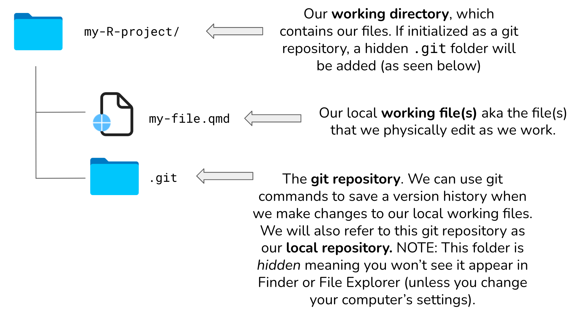
eds212-day2-GHpracticeday2a-vc-gh.qmd)usethis::use_git() (press Enter, then enter the number for YES when prompted)When we initialize our R project as a git repository using usethis::use_git(), a hidden git/ folder is created within that project folder. This hidden .git/ folder is the git repository. As you use git commands (or RStudio’s GUI buttons) to capture versions or “snapshots” of your work, those versions are stored within the .git/ folder. This allows you to access and / or recover any previous versions of your work. If you delete .git/, you delete your project’s history.

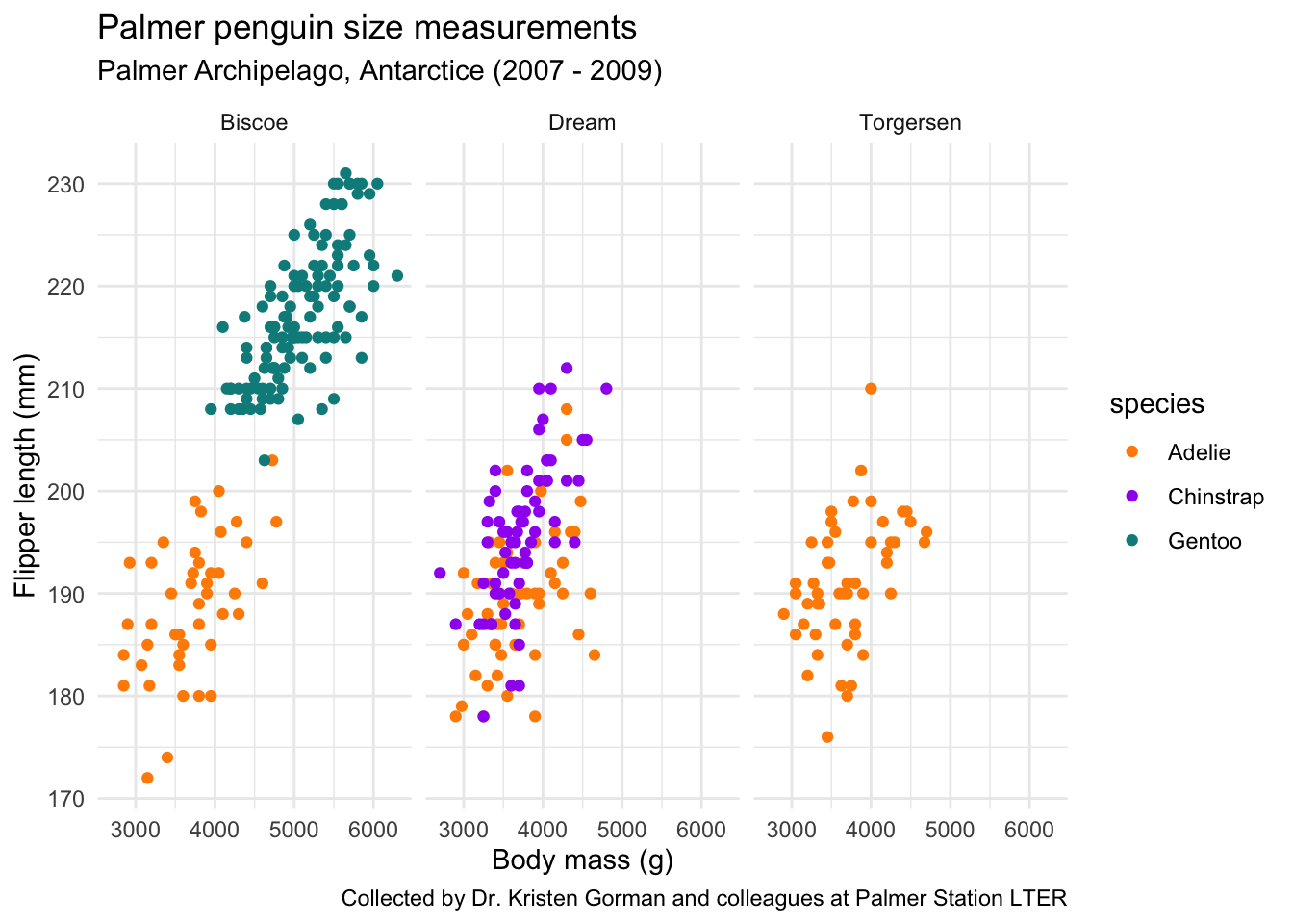
usethis::use_github() (press Enter, then enter the number for YES when prompted).qmd, make some changes (whatever you want). Save. Render (or not…as long as one file changes).Let’s customize a graph a little bit. Here, we’ll use the penguins dataset from the {palmerpenguins} package.
Some extras we’ll learn here are:
# load libraries ----
library(tidyverse)
library(palmerpenguins)

# create plot ----
ggplot(data = penguins, aes(x = body_mass_g, y = flipper_length_mm)) +
  geom_point(aes(color = species)) +
  scale_color_manual(values = c("darkorange","purple","cyan4")) +
  labs(x = "Body mass (g)",
       y = "Flipper length (mm)",
       title = "Palmer penguin size measurements",
       subtitle = "Palmer Archipelago, Antarctice (2007 - 2009)",
       caption = "Collected by Dr. Kristen Gorman and colleagues at Palmer Station LTER") +
  facet_wrap(~island) +
  theme_minimal()
End interactive session 2A