Interactive Session 3A

Credit

This lesson is closely based on the article, Numerically solving differential equations with R.

1. Numerical approximation by hand

We’ll just do this once to reinforce how numerical integration generally works for approximating a particular solution. Given the differential equation:

\[\frac{dP}{dt}=0.4P(0.5 - P)\]

and the initial condition $P(0)=0.2$, approximate the solution $P(t)$ at t = 1, 2.

First, what is $t$, $P$, and $\frac{dP}{dt}$ at $t = 0$?

Here we have the initial condition, $P(0)=0.2$, which we can use to fill out our first row $t$ and $P$ in the table, below
Next, we can use those initial conditions to calculate the slope, $\frac{dP}{dt}$, using our given differential equation: $\frac{dP}{dt} = (0.4)(0.2)(0.5-0.2)$

t	P	dPdt
0	0.2	0.024

Next, approximate the value of $P(t)$ and $\frac{dP}{dt}$ at the next step ($t = 1$)

Importantly, we assume that the slope is continuing at 0.024.

This means that the approximate value of $P(1) = P(0) + (\frac{dP}{dt} * \Delta t)$, therefore, $P(1) = 0.2 + (0.024 * 1) = 0.224$
At that value of $P$, the slope is approximated by $\frac{dP}{dt}=(0.4)(0.224)(0.5 - 0.224) = 0.02473$.

So now, our table is expand to:

t	P	dPdt
0	0.200	0.02400
1	0.224	0.02473

Next, approximate the value of $P(t)$ and $\frac{dP}{dt}$ at the next step ($t = 2$)

Again, we assume that the slope is continuing at the rate determined for the previous time step, 0.02473

We can approximate the value of $P(2) = P(1) + (\frac{dP}{dt} * \Delta t)$, therefore, $P(2) = 0.224 + (0.02473*1) = 0.24873$
At that value of $P$, the slope is approaximated by $\frac{dP}{dt}=(0.4)(0.24873)(0.5 - 0.24873)=0.024999$

Our table is then updated to:

t	P	dPdt
0	0.20000	0.024000
1	0.22400	0.024730
2	0.24873	0.024999

And we could continue doing that for many incremental values of $t$ to get an approximate solution for what the function $P(t)$ looks like. But that would be very tedious. Up next - computer help!

Summary: numerical approximation

There are many different approaches to numerical approximation of solutions for differential equations. This example is meant to give you an idea of how the iterative approximation works generally.

Now, let’s see how much more quickly we can do this with some computer power!

2. Numerical approximation using `deSolve::ode()` (a basic starter)

Create a new R Project named eds212-day3a

Add either an R script or Quarto doc (your choice) to complete the following exercise in.

Let’s say we have a system modeled by:

\[\frac{dC}{dt}=\lambda C^2-3.1\delta\] and we don’t know how to solve this analytically. Let’s use the {deSolve} package in R to help us find a solution numerically, given an initial condition at $C(0)=4.8$ and for parameter values $\lambda = 0.4$ and $\delta=0.06$.

Here’s what a numeric solution looks like with {deSolve}:

# load packages ----
library(deSolve)
library(tidyverse)

First, we’ll make a time sequence that we want to estimate numerical solutions over:

# Create a time sequence ----
time_seq <- seq(from = 0, to = 0.2, by = 0.001)

Then, we’ll store the parameter(s) and initial conditions:

# Set some parameter values (these can change - keep it in mind) ----
parameter_example <- c(lambda = 0.4, delta = 0.06)

# Set the initial conditions ----
init_cond_example <- c(C = 4.8)

Store the differential equation as a function:

# Prepare differential equation(s) as a function, which take three arguments aka inputs (a sequence of time steps, a vector of our initial conditions, and a vector of our parameter values) ----
df_equation_example <- function(time_seq, init_cond_example, parameter_example) {
  
  # using our initial conditions and parameter values ....
  with(as.list(c(init_cond_example, parameter_example)), {
    
    # ... estimate the numerical solutions to this differential equation....
    dCdt = lambda * C^2 - 3.1 * delta
    
    # ...and return a list of approximated solutions calculated at each time step for all equations (here we only have 1 equation that we're solving for)
    return(list(c(dCdt)))
    
  })
}

Breaking down this somewhat odd-looking function structure

The structure of our function body looks a bit different than what we’ve practiced in other recent exercises. Let’s break down the body of our function a bit to better understand what’s happening:

c(init_cond_example, parameter_example) combines the initial conditions and parameter values into a single, named vector (both init_cond_example and parameter_example are named vectors)
as.list(c(init_cond_example, parameter_example)) converts our named vector into a list, where each element can be accessed by name
- for example, we can access the delta variable in our list using the syntax, (as.list(c(init_cond_example, parameter_example)))$delta
- we cannot access delta by name when in vector format (e.g. c(init_cond_example, parameter_example)$delta)
with(as.list(c(init_cond_example, parameter_example)), { ... }) evaluates the block of code (inside {}) in an environment where the names in our list (i.g. C, lambda, delta) are treated as variables and can be directly referenced by name

Use deSolve::ode() to approximate the solution numerically:

# Find the approximate solution using `deSolve::ode()` ----
approx_df_example <- ode(y = init_cond_example,
                         times = time_seq, 
                         func = df_equation_example, 
                         parms = parameter_example)

# Check the class ----
class(approx_df_example)

[1] "deSolve" "matrix"

# We really want this to be a data frame for plotting (more to come in EDS 221) ----
approx_df_example <- data.frame(approx_df_example)
class(approx_df_example) # you might also consider looking at it using `View(approx_df_example)`

[1] "data.frame"

# Plot it ----
ggplot(data = approx_df_example, aes(x = time, y = C)) +
  geom_point(size = 0.1)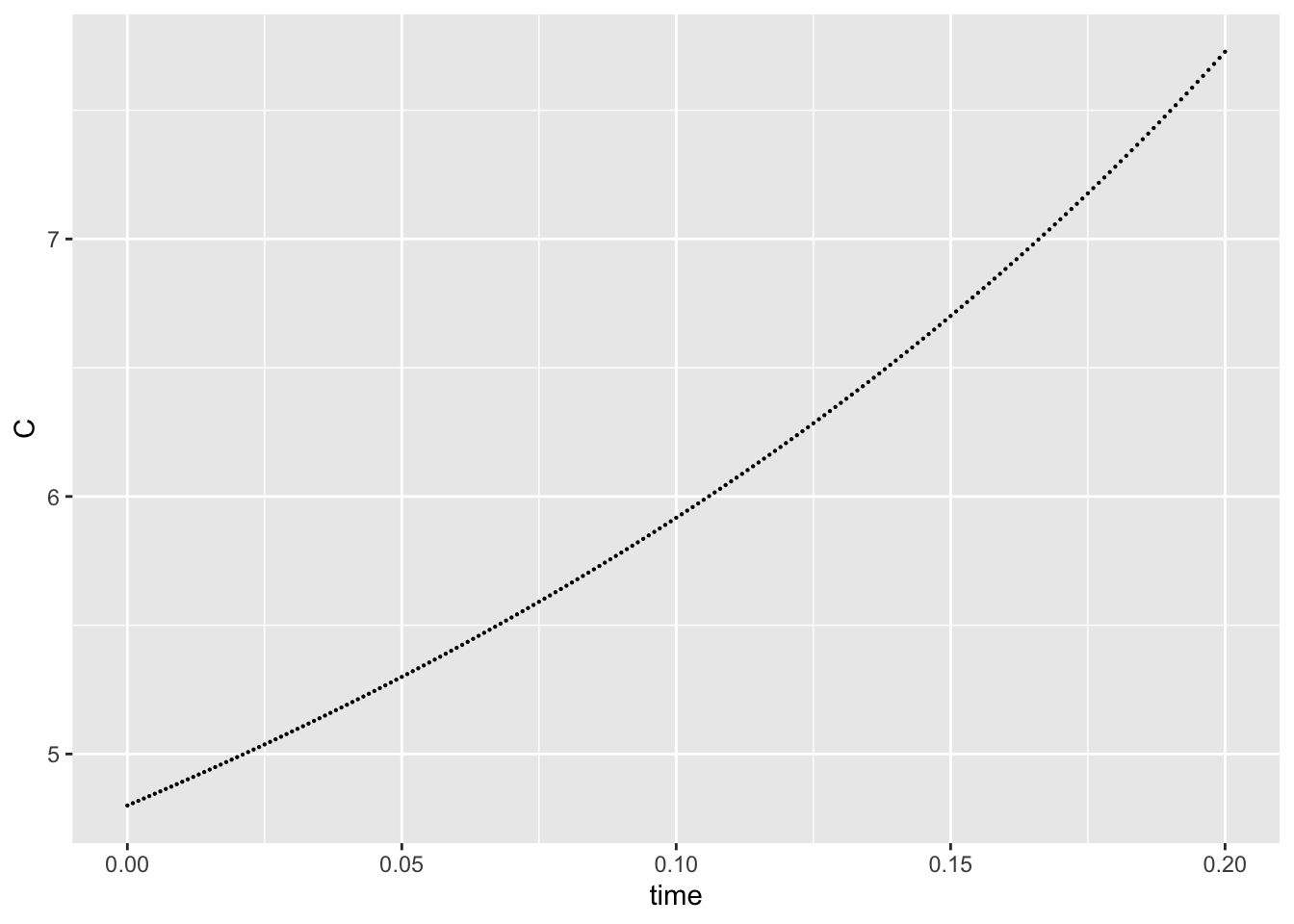

Now let’s try it for something a bit more interesting!

3. Fork and clone a repo

In this session, you will use existing code in a public repo on GitHub that approximates the solution to the Lotka-Volterra equations.

You will make your own copy of the repo by forking it. By making a fork, you create a copy that you can work in separately.

Visit: https://github.com/EDS-212-Essential-Math/lotka-volterra-example
Press the Fork button to make a copy - note the repo is now copied into your account
So far, you just have a remote copy. We need a local copy of the repo, that we can work in locally. We do that by cloning a repo. Press the Code button in YOUR copy of the repo. Copy the URL to your clipboard.
Go back to RStudio. Create a new project WITH version control. Paste the URL where prompted, then choose the destination for your new project. Create the project.
You should see that the materials from the remote repo now exist locally in a version controlled R project. Yay!

4. Run existing code

The repo contains a single .qmd (lotka-volterra.qmd), with information and code to numerically approximate solutions to the Lotka-Volterra equations and make a graph.

Open the .qmd and render. We will talk through the code together. A couple of things to note:

When you knit, the .html doesn’t appear in the git pane. Why?
How does the numerical approximation change if you update the initial conditions? The parameter estimates?
Try making changes, then stage > commit > push back to your remote repo. Make sure the changes appear there.
Congratulations! You’ve adding forking and cloning to your git toolkit.

5. Command line intro + git

Here, we’ll learn a few basic commands to talk with your computer through the command line to navigate around and do some git stuff outside of RStudio.

Some basics:

Open the Terminal (Mac) or Git Bash (Windows) (outside of RStudio)
Use pwd to see where your Terminal currently sees the working directory
Use ls to see the contents of the directory
Use cd to change to a different downstream directory
Use .. to go back upstream

Now for git:

Return to RStudio and switch from the Console tab to the Terminal tab in your lotka-volterra-example project
Use pwd to see your current working directory (it should be your project’s root directory!)
Use git status to see the current git status
Make a change to the .qmd in your project and save
Run git status to see any newly added or modified files (they’ll appear red)
Use git add filename.qmd to stage it (git add . will stage everything)
Run git status again to see all staged files (they should now appear green)
Use git commit -m "a commit message" to commit to local repo
Use git status again to check status
Use git pull to pull
Use git push to push changes
Check with git status

End interactive session 3A

Interactive Session 3A

1. Numerical approximation by hand

First, what is \(t\), \(P\), and \(\frac{dP}{dt}\) at \(t = 0\)?

Next, approximate the value of \(P(t)\) and \(\frac{dP}{dt}\) at the next step (\(t = 1\))

Next, approximate the value of \(P(t)\) and \(\frac{dP}{dt}\) at the next step (\(t = 2\))

Summary: numerical approximation

2. Numerical approximation using `deSolve::ode()` (a basic starter)

3. Fork and clone a repo

4. Run existing code

5. Command line intro + git

Some basics:

Now for git:

1. Numerical approximation by hand

First, what is \(t\), \(P\), and \(\frac{dP}{dt}\) at \(t = 0\)?

Next, approximate the value of \(P(t)\) and \(\frac{dP}{dt}\) at the next step (\(t = 1\))

Next, approximate the value of \(P(t)\) and \(\frac{dP}{dt}\) at the next step (\(t = 2\))

Summary: numerical approximation

2. Numerical approximation using deSolve::ode() (a basic starter)

3. Fork and clone a repo

4. Run existing code

5. Command line intro + git

Some basics:

Now for git:

2. Numerical approximation using `deSolve::ode()` (a basic starter)