End interactive session 4A
# Make a sequence of values from 1 - 10 ----
my_values <- seq(from = 1, to = 10, by = 1)

# Look at it (always) ----
my_values
[1] 1 2 3 4 5 6 7 8 9 10Linear algebra continued: matrices in R and a Leslie Matrix example
eds212-day4a, with a READMEr-matrices.qmdA matrix contains data of a single class (usually numbers). Which means that we can think of the contents of a matrix as a single sequence of values, that are constrained (wrapped) to the specified dimensions of the matrix.
For example, let’s say we have 10 values:
# Make a sequence of values from 1 - 10 ----
my_values <- seq(from = 1, to = 10, by = 1)
# Look at it (always) ----
my_values [1] 1 2 3 4 5 6 7 8 9 10Now, we can convert this into a matrix by letting R know how many rows these values should be “wrapped” into (the default is to populate by column…see documentation, and always look at what you’ve created):
# Convert to matrix ----
my_matrix <- matrix(data = my_values, nrow = 2, ncol = 5, byrow = TRUE)

# Check it out ----
my_matrix
[,1] [,2] [,3] [,4] [,5]
[1,] 1 2 3 4 5
[2,] 6 7 8 9 10Try some other variations to make a matrix from my_values to test it out. What happens if you don’t have enough elements in the matrix to contain your vector?
For example:
Warning in matrix(data = my_values, nrow = 2, ncol = 3, byrow = TRUE): data
length [10] is not a sub-multiple or multiple of the number of columns [3]
[,1] [,2] [,3]
[1,] 1 2 3
[2,] 4 5 6What happens if your matrix has more elements than your vector?
For example:
Warning in matrix(data = my_values, nrow = 3, ncol = 4, byrow = TRUE): data
length [10] is not a sub-multiple or multiple of the number of rows [3]
[,1] [,2] [,3] [,4]
[1,] 1 2 3 4
[2,] 5 6 7 8
[3,] 9 10 1 2So…always, always, always look at what you’ve created.
Scalar multiplication of a matrix is straightforward: just use the multiply operator (*):
Addition/subtraction requires matrices of the same dimension. Let’s make another 2x5 matrix:
# Make 2x5 matrix ----
my_values2 <- seq(from = 21, to = 30)
my_matrix2 <- matrix(my_values2, nrow = 2, byrow = TRUE)

# Check it out ----
my_matrix2
[,1] [,2] [,3] [,4] [,5]
[1,] 21 22 23 24 25
[2,] 26 27 28 29 30Add the two matrices:
Similarly for subtraction:
As we saw in lecture, matrix multiplication is a bit more complicated (dot products of rows by columns become elements in the resulting matrix). Here’s a reminder:

We multiply matrices in R using the same operator as the dot product for vectors: %*%
For example:
# Make a couple of 2x2 matrices ----
cats <- matrix(data = c(0,4,3,1), nrow = 2, byrow = TRUE)
dogs <- matrix(data = c(6,-3,0,2), nrow = 2, byrow = TRUE)

# Look at them ----
cats
[,1] [,2]
[1,] 0 4
[2,] 3 1 [,1] [,2]
[1,] 6 -3
[2,] 0 2 [,1] [,2]
[1,] 0 8
[2,] 18 -7Confirm that this is correct by doing the matrix multiplication by hand.
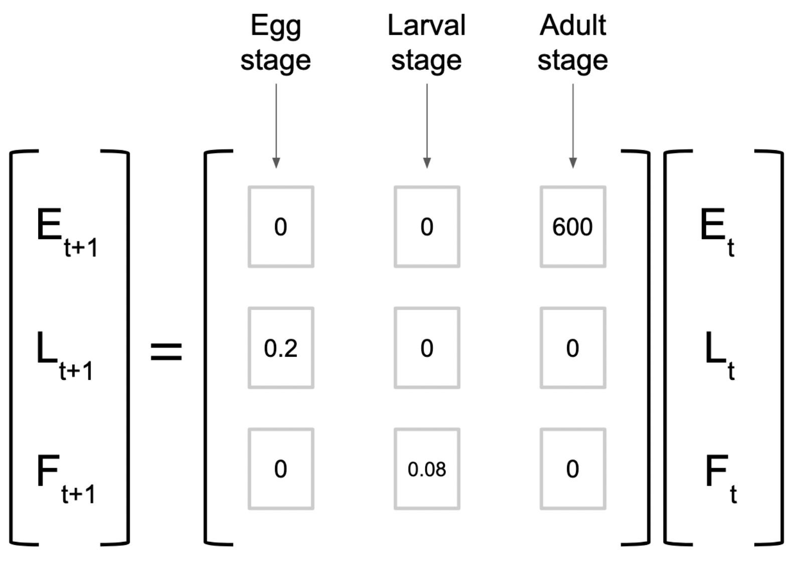
In lecture, we considered a Leslie matrix for an insect with three life stages, that looked like this:

Let’s say we start with 12000 eggs, 700 larvae, and 500 female adults. Create a vector containing those initial values:
Reminder: this means we’ll take the dot product of our projection matrix, and the lifestage populations.
       [,1]
[1,] 300000
[2,]   2400
[3,] 56\[insects\;Y_2 = \begin{bmatrix} 0&0&600 \\ 0.2&0&0 \\ 0&0.08&0 \end{bmatrix} \times \begin{bmatrix} 1200 \\ 700 \\ 500 \end{bmatrix} = \begin{bmatrix} (0\times12000)+(0\times700)+(600\times500) \\ (0.2\times12000)+(0\times700)+(0\times500) \\ (0\times500)+(0.08\times700)+(0\times500) \end{bmatrix} = \begin{bmatrix} 300,000 \\ 2,400 \\ 56 \end{bmatrix}\]
# Populations by lifestage at year 2 ----
insect_y2 <- insect_leslie %*% insect_y1

# Check it out ----
insect_y2
[,1]
[1,] 33600
[2,] 60000
[3,] 192# Populations by lifestage at year 3 ----
insect_y3 <- insect_leslie %*% insect_y2
# Check it out ----
insect_y3 [,1]
[1,] 115200
[2,] 6720
[3,] 4800# Populations by lifestage at year 4:
insect_y4 <- insect_leslie %*% insect_y3
# Check it out ----
insect_y4 [,1]
[1,] 2880000.0
[2,] 23040.0
[3,] 537.6Yes! Keep this in mind for EDS 221 when we start with iteration (for loops)!
You have collected information about a type of tree. There are three life stages: seeds (S), juvenile (J) and adult (A). Juvenile trees don’t produce seeds. Adults produce 5000 seeds each year. 10% of seeds produced become seedlings (juveniles), and 6% of seedlings go on to become adults. 95% of adult trees survive each year.
It’s helpful to begin by drawing the Leslie matrix by hand:
\[\begin{bmatrix} S_{t+1} \\ J_{t+1} \\ A_{t+1} \end{bmatrix} = \begin{bmatrix} 0&0&5000 \\ 0.1&0&0 \\ 0&0.06&0.95 \end{bmatrix} \times \begin{bmatrix} S_t\\ J_t \\ A_t \end{bmatrix}\]
Where:
\[\begin{bmatrix} S_{t0}\\ J_{t0} \\ A_{t0} \end{bmatrix} = \begin{bmatrix} 5000\\ 0 \\ 0 \end{bmatrix}\]
# Make the projection matrix ----
tree_leslie <- matrix(c(0, 0, 5000, 0.10, 0, 0, 0, 0.06, 0.95), nrow = 3, ncol = 3, byrow = TRUE)

# Check it out (it should look just like the one you drew!) ----
tree_leslie
[,1] [,2] [,3]
[1,] 0.0 0.00 5000.00
[2,] 0.1 0.00 0.00
[3,] 0.0 0.06 0.95Make some projections:
You may choose to do so via the Git tab + buttons or via the RStudio Terminal.
End interactive session 4A