EDS 212: Day 3, Lecture 1

Integration and differential equations - reading, understanding, solving numerically in R

---

August 7^th, 2024

Integration fundamentals - initial conditions for particular solutions

---

If your lemonade stand makes $200/yr, how much money do you make from your lemonade stand over 4 years?

Do you know how much total money you have in your bank account from the information above?

Big takeaway: We can know how much an amount changes without knowing the absolute amount in our bucket. But if we want to know the absolute amount, then we need an initial condition!

Integration blitz

---

Integration: A tool to get from rates back to amounts (e.g. \(\frac{df}{dx}\rightarrow f(x)\))

We can think of it as antiderivation.

• If \(f(x)=x^2\), then \(\frac{df}{dx}=2x\)
• If \(\frac{df}{dx} = 2x\), then \(f(x)=?\)

Question: if you don’t know the original function and only have an expression for the rate (slope), then from the slope can you know the exact solution?

• \(f(x)=x^2\)

• No because we have no idea the value of the constant of integration. Without additional information, such as an initial condition or a specific value of the function at a particular point, you cannot determine the exact value of \(C\)

One rule for practice: the power rule for integration

---

\[\int{x^n}dx=\frac{x^{n+1}}{n+1} + C\]

Example: If \(\frac{df}{dx}=3.8x^2-2.1\):

1. Find a general expression for \(f(x)\)

2. Given the initial condition \(f(1.4)=5.9\), find the particular solution for \(f(x)\)

1. \(\frac{df}{dx}=3.8x^2-2.1\)

• \(f(x) = \int(3.8x^2-2.1)dx\)
• \(f(x) = 3.8 \frac{x^3}{3} - 2.1x +C\)
• \(f(x) = 1.267{x^3} - 2.1x +C\)

2. We need to solve for \(C\)!

• \(5.9 = 3.8 \frac{1.4^3}{3}-(2.1)(1.4)+C\)
• \(5.9 = 2.48-2.94+C\)
• \(5.9 = 0.54+C\)
• \(C = 5.36\)
• So, the particular solution for \(f(x)\) is \(f(x) = 1.267{x^3} - 2.1x + 5.36\)

Introduction to differential equations & solving them

---

A differential equation is an equation containing a differential expression. So it describes rates, often related to a function containing our variables of interest.

For example:

\[\frac{df}{dt}=3.2-f(t)\]

is a differential equation because it contains both a the function \(f(t)\) and it’s derivative, \(\frac{df}{dt}\).

Explain how the rate of change could depend on the value of the function e.g. population growth

Differential equations: terms

---

• Ordinary differential equation (ODE): Does not contain partial derivatives

\[\frac{df}{dt}=3.2-f(t)\]

• Partial differential equations (PDE): Does contain partial derivatives

\[\frac{\partial B}{\partial t}= \alpha B+0.31x-21.6\]

Order of an ODE

---

Order: The order of a differential equation is the highest order for any differential expression in the equation

Example:

\(\frac{df}{dt}=3.2-f(t)\) is a first order ordinary differential equation

Example:

\(\frac{\partial^3x}{\partial t^3}=2x-4.5\frac{\partial x}{\partial t}\) is a third order partial differential equation

Practice:

---

Use the terms from the previous slide to describe the following different equations:

\[\frac{\partial^2f }{\partial x^2}=1.4\times10^{-3}f(x)+5.2\]

\[2.9t^2 - \alpha B=\frac{dB}{dt}\]

\[\frac{dC}{dt}=4.1C-8.0\]

Example: Lotka-Volterra (predator-prey) equations

---

Prey: \(\frac{dV}{dt}=r V-\alpha VP\)

Predator: \(\frac{dP}{dt}=\beta VP - qP\)

Where:

• \(V\) is number of prey (e.g. rabbits)
• \(P\) is number of predators (e.g. wolves)
• \(r, \alpha, \beta, q\) are positive parameters

• \(r\): intrinsic rate of increase
• \(\alpha\): capture efficiency of predators (i.e. effect of a predator on per capita growth rate of prey population)
  • the larger \(\alpha\) is, the more the per capita growht rate of a prey population is depressed by the addition of a single predator (e.g. baleen whales feeding on plankton vs. web-building spider capturing a mosquito)
• \(\beta\): a measure of conversion efficiency (i.e. the ability of predators to convert each new prey ite m into additional per capita growth rate for the predator population)
  • \(\beta\) is high when a single prey item is high value (e.g. a moose prey to wolf predator vs. a seed to a bird)
• \(q\): per capita death rate (these predators are extreme specialists with no alternative prey sources; so if prey are absent, the predator population declines exponentially)

Thinking about differential equations: break it down

---

Instantaneous rate of change in prey population size:

\[\frac{dV}{dt}=r V-\alpha VP\]

Where:

• \(V\) is number of prey (e.g. rabbits)
• \(P\) is number of predators (e.g. wolves)
• \(r, \alpha, \beta, q\) are positive parameters

What do the different pieces of the equation mean?

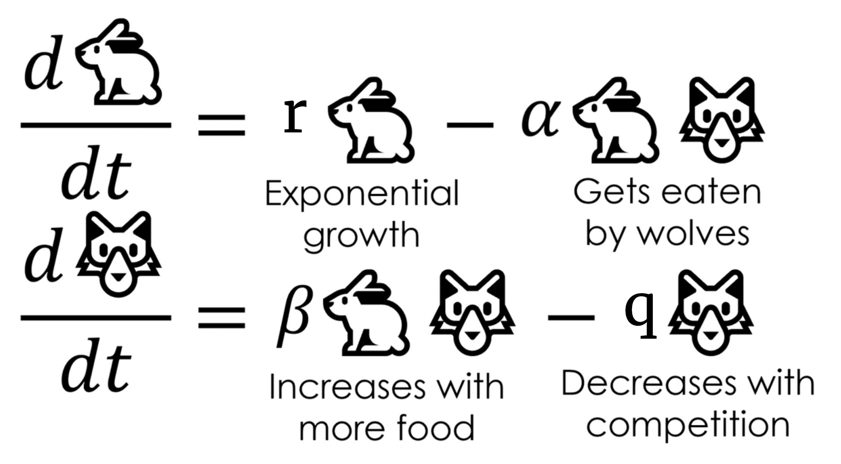
Interpretation of prey equation:

---

\[\frac{dV}{dt}=r V-\alpha VP\]

The pieces:

• \(\frac{dV}{dt}\): Rate of growth / decline in prey abundance
• \(r V\): Population growth (without loss due to predation (assumes predators are the only force limited the growth of the prey population), where \(r\) is the intrinsic rate of increase)
• \(-\alpha VP\): Population loss due to predation (where \(\alpha\) is the capture efficiency of the predator)

Interpretation of predator equation:

---

\[\frac{dP}{dt}=\beta VP - q P\]

The pieces:

• \(\frac{dP}{dt}\): Rate of growth / decline in predator population
• \(\beta VP\): Predator population growth (where \(\beta\) is a measure of conversion efficiency, i.e. the ability of predators to convert each new prey into additional per capita growth rate for the predator population)
• \(-q P\): Predator population loss (where \(q\) is the per capita death rate; positive population growth only happens when prey are present)

Or, in pictures:

---

Now we know the rates of change for both populations, but what we still want to know is the actual numbers through time.

Finding \(V(t)\) and \(P(t)\)?

---

Some differential equations can be solved analytically:

---

\[\frac{dy}{dx}=y\]

Separate variables and integrate both sides:

\[\int\frac{1}{y}dy=\int1dx\]

Yielding:

\(ln(y)=x\) or \(y=e^x\)

Numerical solutions versus analytical solutions

---

“Differential equations textbooks are cookbooks that give you lots of suggestions about approaches, but there are lots of differential equations (DEs) that simply don’t have analytic solutions — that is, solutions that you can write down. These equations can only be solved numerically…”

- Dr. Liz Bradley (CS, University of Colorado)

Solving differential equations numerically

---

Find approximate solutions to differential equations when finding an analytical solution would be really challenging (…which is pretty often).

Instead, computers can numerically approximate solutions by predicting nearby values based on the slope.

There are many methods for solving differential equations numerically. Here we’ll just get a little flavor.

The general process (many methods) exist

---

From the expression for slope and using an initial condition & parameter estimates, start at one endpoint and incrementally calculate values of the solution from the slope expression until reaching the other endpoint.

This means that the approximate solution is found by approximating values of the solution at equal intervals of the independent variable (often, time).

Example: numerical approximation of DE solution

---

Let’s say that we have a differential equation, \(\frac{dP}{dt}=0.4P(0.5 - P)\), and we don’t know how to solve analytically for \(P(t)\). Using the initial condition \(P(0)=0.2\), let’s numerically estimate the solution.

We’ll create a table that estimates \(P\) at increments of \(t\) based on an approximation of the slope estimate \(\frac{dP}{dt}\) . WHAT?

It’s OK, follow along by hopping over the Interactive Session 3A (and afterwards, we’ll learn how to use the {deSolve} package in R to make this process a lot easier).